Correction of Terrestrial LiDAR Data Using a
Hybrid Model
Wallace MUKUPA, China, Gethin Wyn ROBERTS,
United Kingdom, Craig Matthew HANCOCK, China, Khalil AL-MANASIR, China

Wallace Mukupa
1)
This paper is a peer review paper that was presented at the FIG Working
Week 2017. Wallace Mukupa received a ph.d. grant from FIG Foundation in
2016 and one of the results is this peer review paper. In this paper, a
hybrid method for correcting intensity data is presented.
Read
Wallace Mukupa's report about the Ph.D. grant and from the FIG Working Week
SUMMARY
The utilization of Terrestrial Laser Scanning (TLS) intensity data in
the field of surveying engineering and many other disciplines is on the
increase due to its wide applicability in studies such as change
detection, deformation monitoring and material classification.
Radiometric correction of TLS data is an important step in data
processing so as to reduce the error in the data. In this paper, a
hybrid method for correcting intensity data has been presented. The
proposed hybrid method aims at addressing two issues. Firstly, the issue
of near distance effects for scanning measurements that are taken at
short distances (1 to 6 metres) and secondly, it takes into account the
issue of target surface roughness as expounded in the Oren-Nayar
reflectance model. The proposed hybrid method has been applied to
correct concrete intensity data that was acquired using the Leica
HDS7000 laser scanner. The results of this proposed correction model are
presented to demonstrate its feasibility and validity.
1. INTRODUCTION
Correction of intensity data is essential due to systematic effects
in the LiDAR system parameters and measurements and in order to ensure
the best accuracy of the delivered products (Habib et al., 2011). The
whole aim of radiometric correction is to convert the laser returned
intensity recorded by the laser scanner to a value that is proportional
to the object reflectance (Antilla et al., 2011). This correction of
intensity data is still an open area of investigation and this is the
case because even though a couple of researchers have studied the
subject of TLS intensity correction for instance, a standard correction
method that can be applicable for all the various types of laser
scanners is non-existent (Penasa et al., 2014). Such a scenario is also
explained by some of the laser scanning research work that are still
being published without the intensity data having been corrected (Krooks
et al., 2013). However, in Tan and Cheng (2015), it is purported that
the proposed intensity correction method is suitable for all TLS
instruments. In the case of Airborne Laser Scanning (ALS), the subject
of intensity data correction has an old history compared to TLS and this
has been reported by researchers such as Kaasalainen et al. (2011).
It has been reported that the effect of the measurement range
(distance) on the intensity data depends on several parameters. In the
case of TLS, the effects of the range tend to depend on the instrument
especially when measurements are taken at close range to the target. The
effects of the range on TLS intensity or the dependence of the received
power as a function of the range is proportional to 1/R2 (R = range) in
the case of extended diffuse targets (Jelalian, 1992). This implies that
the whole laser footprint is reflected on one surface and it has
Lambertian scattering properties. However, non-extended diffuse targets
exhibit different range dependencies. For instance, point targets (e.g.
a leaf) with an area smaller than the footprint are range independent
and targets with linear physical properties (e.g. wire) are linear range
dependent. Therefore, the range dependency becomes 1/R4 for targets
smaller than laser footprint size and 1/R3 for linear targets (Vain and
Kaasalainen, 2011).
According to Krooks et al. (2013), different scanners have different
instrumental effects on the measured intensity and this implies that it
is prudent to study each scanner individually. Instrumental effects have
been reported to affect the intensity recorded for TLS instruments. Even
though distance has been predicted to follow the range squared inverse
(1/R2) dependency for extended targets based on the physical model
(radar equation), in practical applications this prediction is
inapplicable at all ranges because of TLS instrumental modifications
that are designed to enhance the range measurement determination (Holfe
and Pfeifer, 2007; Balduzzi et al., 2011; Antilla et al., 2011). In a
similar vein, Kaasalainen et al. (2011) state that the knowledge of the
TLS instrument as to whether it has near-distance reducers or
logarithmic amplifiers in the case of small reflectance is of cardinal
importance in an attempt to know the distance effects and the extent to
which the measured intensity is affected by instrumental effects. In
Kaasalainen et al. (2009a) it is has been reported that measurement of
the intensity taken at short ranges, 1m in this case have been
significantly affected at such near distances by brightness reducers.
The effects of the incidence angle on the intensity are related to
the scanned target object in terms of its surface structure and
scattering properties (Krooks et al., 2013). In terms of the rugosity of
the target, macroscopic irregularities of the order of mm to cm size and
almost the same size as the laser footprint, neutralize the effects of
the incidence angle on the intensity. This is so because there are
always elements on the surface of the target that are perpendicular to
the incident laser beam (Kaasalainen et al., 2011). In a similar vein
Penasa et al. (2014) states that the effects of the scattering angle can
be neglected if the surface roughness of the target is comparable with
the laser spot size. Other studies for instance Kaasalainen et al.
(2009b) showed that the significance of the angle of incidence only
becomes an important parameters when it is greater than 20° for several
materials. The strength of the signal that the scanner receives is
dependent on the backscattering properties of the target scanned (Shan
and Toth, 2009). If the surface backscattering the laser is an extended
target and a Lambertian reflector, the backscatter strength in the
angular domain depends entirely on the incidence angle.
Different TLS intensity correction models have been proposed and some
methods are based on the physical model (laser range equation) whereas
others are modified versions of the physical model and some are data
driven. For instance in Balduzzi et al. (2011) the modified radar range
equation was used to correct the intensity data. It is reported that the
laser scanner (FARO LS880) which was used has an intensity filter and
with the assumption that this filter has only an impact on the intensity
variations due to distance, the range squared inverse law was replaced
by a device specific distance function and then a logarithmic function
was applied. In Kaasalainen et al. (2008), an important consideration
was the effect of the logarithmic amplifier of the FARO LS HE80 for small
reflectance. The logarithmic correction was calibrated by fitting an
exponential function.
In Penasa et al. (2014) an intensity correction approach for distance
effects and exclusive of other variables such as incidence angle or
atmospheric losses is presented. The correction approach did not apply
the radar equation instead it is stated that the correction was based on
estimating a correcting intensity-distance function on an appropriate
reference point cloud via a Nadaraya–Watson regression estimator. In
Blaskow and Schneider (2014) an intensity correction approach is
presented which involves polynomial approximation and static correction
model. Under the polynomial approximation, the intensity-distance curves
were functionalised as basis for the static correction model and the
Spectralon target data served as reference. Pfeifer et al. (2007)
investigated data driven models and a function, F(ρ, α, r) was sought to
predict the intensity value from range (r), reflectivity (ρ) and
incidence angle (α). To correct the intensity for the effects of target
reflectivity and incidence angle, different functions were tested. The
function which brought the curves to the closest overlap was (ρ
cos(α))-0.16 and all intensity values were then multiplied by this
function to remove the influence of target reflectivity and angle of
incidence. Two linear functions were then fitted to correct the
intensity for distance effects. In Franceschi et al. (2009) a study was
undertaken that focused on using TLS intensity data to discriminate
between marls and limestone, the corrected intensity was taken to be
related and proportional to the target reflectivity and an assumption
was made that the scanned objects were Lambertian reflectors.
In Fang et al. (2015) an intensity correction method is presented
based on estimating the laser transmission function so as to determine
the ratio of the input laser signal between the limited and the
unlimited ranges and then integrating this ratio in the radar range
equation in order to correct the intensity data near distance effects.
Tan and Cheng (2015) developed a model to correct the effects of the
angle of incidence and the distance on the intensity data. The proposed
correction model is approximated by a polynomial series based on the
Weierstrass approximation theory and an approach to estimating the
specific parameters is presented. Using a similar approach, Tan et al.
(2016) proposed an intensity correction method for distance effects
where the range squared inverse law as described in the radar equation
and the ALS range correction methods was replaced by a polynomial
function of distance. Zhu et al. (2015) investigated the use of TLS
intensity data to detect leaf water content and an intensity correction
method is described where firstly a reflection model was employed to get
rid of specular reflection which was as a result of leaf surface at
perpendicular angle and then reference targets were utilised to correct
the effects of the angle of incidence.
In view of the above, this study aimed at correcting the TLS returned
intensity for concrete by looking at methods of modelling the variables
that have an effect on the intensity values of the laser in this case
the effects of the measurement range and incident angle since the
experiment was carried out in a controlled environment. The focus of the
investigation was to use existing models of laser behaviour to develop a
correction model for TLS intensity data that is also capable of
addressing near-distance effects and surface roughness of the target
since not all objects are perfect Lambertian reflectors. The proposed
hybrid intensity correction method is based on the radar equation
(Jelalian, 1992), near-distance correction model (Fang et al., 2015) and
the Oren-Nayar reflectance model (Carrea et al., 2016). These existing
models and the development of a hybrid intensity correction model are
explained in detail in the data processing section. A description of the
experimental procedure for testing the proposed hybrid method for
correcting intensity data is provided and the results of this correction
model are presented to demonstrate the feasibility and validity of the
method.
2. EXPERIMENTAL PROCEDURE
2.1 Target Objects: Concrete Specimens
Prismatic concrete beams (Fig. 1) were used as scanning target
objects mainly because this is part of an on-going project investigating
the use of laser intensity for the assessment of fire-damaged concrete.
Since surface roughness of the scanned object was of interest in this
study, it is worth mentioning that the concrete consisted of fine
aggregate (river sand) with a maximum grain size of 5 mm and crushed
siliceous coarse aggregate with a diameter ranging from 5 to 20 mm. For
easy identification, the concrete specimens were labelled as: Block C,
Block 1, Block 2, Block 3 and Block 4.
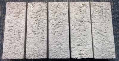
Fig. 1: Concrete specimens
2.2 Scanning Room and Equipment
The experiments were conducted under controlled laboratory conditions.
The factors affecting the returned intensity under such conditions are
the scanning geometry and the instrumental effects. Since the
experiments were carried out in a controlled environment and at short
range (1 to 6m), atmospheric losses were neglected. The Leica HDS7000
laser scanner (Fig. 2) was used to scan the concrete specimens and the
technical specifications of this scanner are as presented in Table 1
below.
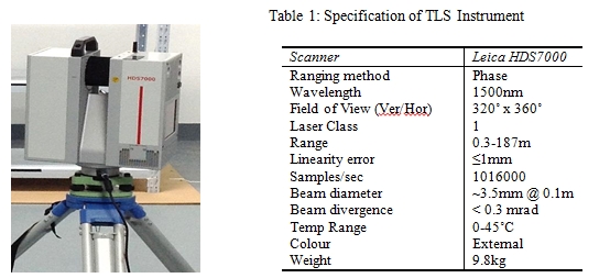
Fig 2: HDS7000 Laser Scanner
Source: Leica Geosystems (2012)
2.3 Measurement Setup and Data Acquisition
The measurement distances between the HDS7000 scanner and the target
objects (concrete specimens) were ranging from 1 to 6 metres and the
total station was utilized in marking out the scanning distances. The
steel frame where the blocks were placed was levelled using a spirit
level and then the distance to the prism placed right on the edge and
centre of the steel frame was measured. Distances up to 6m in steps of
1m were measured using a total station so as to have scans taken from
well-known accurate distances. The geometry of the experiment in terms
of scanning measurement setup is shown in Fig. 3.
F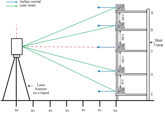
Fig. 3: Laser scanner and blocks at different levels on a frame (Letters
A, B, C, D and E stand for shelf levels).
With reference to Fig. 3, the planar surface of each concrete block was
properly aligned with the frame edge with the aid of a mark which was
made on the centre of the block and the frame too. These measures were
carried out so as to position each concrete block at approximately the
same required distance from the scanner for each respective scanning
session. Independent measurements using a steel rule and tape were
carried out to ensure that each concrete block was accurately oriented.
The experiment was set-up this way in order to only focus on the
scanning geometry which consists of the angle of incidence and the range
between the scanner and the target object (Krooks et al., 2013;
Kaasalainen et al., 2011) as the factor influencing the poor laser
returned signal. The concrete blocks were placed at different heights on
shelves of the steel frame with the control block on the centre shelf at
the same height as the scanner with its front face approximately
vertical and perpendicular to ensure that scanning was done at roughly
normal angle of incidence. The scanning parameters used in the
experiments involved super high resolution and a normal quality.
3. DATA PROCESSING
3.1 Scan Data Pre-processing
The HDS7000 scans were converted to text files (.pts format) using the Z
+ F laser control software instead of the Leica Cyclone software as it
has been reported for instance in Kaasalainen et al. (2011) that
this software scales the intensity so as to accentuate visualisation.
The scans which were converted to text files contained the geometric
data in terms of X, Y and Z coordinates in a Cartesian coordinate system
as well as radiometric data i.e. the intensity values for the 3D
coordinates. The intensity values of data converted to text files were
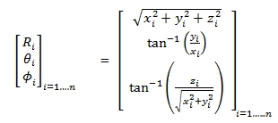
ranging from -2047 to +2048. The output Cartesian coordinates can be
converted to spherical (range, zenith and azimuth angles) coordinates
based on a zero origin for the TLS instrument as described in Eq. (1)
(Soudarissanane et al., 2009):
 3.2 Intensity Data Correction
The proposed hybrid intensity correction method consists of two parts,
namely the near-distance correction model in Fang et al. (2015) and the
Oren-Nayar correction model described in Carrea et al. (2016). In
principle, the hybrid intensity correction method has a basis in the
radar (range) equation (Eq. (2)) and so an overview of this equation is
presented and then it is followed by the correction for near-distance
effects and the Oren-Nayar reflection model. The radar (range) equation
(Eq. (2)) consists of three main components and these are: the sensor,
the target and the environmental parameters which diminish the amount of
power transmitted. Importantly, this equation (Eq. (2)) has been applied
as a physical model for the correction of laser intensity data (Yan and
Shaker, 2014) in several studies where the equation has been applied
either as it is or in a modified form.
3.2 Intensity Data Correction
The proposed hybrid intensity correction method consists of two parts,
namely the near-distance correction model in Fang et al. (2015) and the
Oren-Nayar correction model described in Carrea et al. (2016). In
principle, the hybrid intensity correction method has a basis in the
radar (range) equation (Eq. (2)) and so an overview of this equation is
presented and then it is followed by the correction for near-distance
effects and the Oren-Nayar reflection model. The radar (range) equation
(Eq. (2)) consists of three main components and these are: the sensor,
the target and the environmental parameters which diminish the amount of
power transmitted. Importantly, this equation (Eq. (2)) has been applied
as a physical model for the correction of laser intensity data (Yan and
Shaker, 2014) in several studies where the equation has been applied
either as it is or in a modified form.
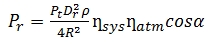
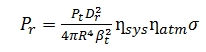 Where Pr is the received power, Pt is the power transmitted, Dr is the
receiver aperture, R is the range between the scanner and the target, βt
is the laser beam width, σ is the cross-section of the target, ηsys and
ηatm are system and atmospheric factors respectively. The cross-section
σ can be described as follows (Hӧfle and Pfeifer, 2007):
Where Pr is the received power, Pt is the power transmitted, Dr is the
receiver aperture, R is the range between the scanner and the target, βt
is the laser beam width, σ is the cross-section of the target, ηsys and
ηatm are system and atmospheric factors respectively. The cross-section
σ can be described as follows (Hӧfle and Pfeifer, 2007):
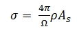 Where Ω is the scattering solid angle of the target, ρ is the
reflectivity of the target and As the area illumination by the laser
beam. Under the following assumptions Eq. (3) can be simplified. First,
the entire footprint is reflected on one surface and the target area
illumination As is circular, hence defined by the range R and laser beam
width β. Secondly, the target has a solid angle of π steradian (Ω = 2π
for scattering into half sphere). Thirdly, the surface has Lambertian
scattering charateristics. If the incidence angles are greater than zero
(α > 0°), σ has a proportionality of cos α (Hӧfle and Pfeifer, 2007):
Where Ω is the scattering solid angle of the target, ρ is the
reflectivity of the target and As the area illumination by the laser
beam. Under the following assumptions Eq. (3) can be simplified. First,
the entire footprint is reflected on one surface and the target area
illumination As is circular, hence defined by the range R and laser beam
width β. Secondly, the target has a solid angle of π steradian (Ω = 2π
for scattering into half sphere). Thirdly, the surface has Lambertian
scattering charateristics. If the incidence angles are greater than zero
(α > 0°), σ has a proportionality of cos α (Hӧfle and Pfeifer, 2007):
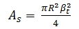 Substituting As in Eq. (4) into Eq. (3) leads to:
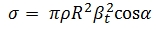 Substituting Eq. (5) into Eq. (2) results into a squared range which is
inversely related to the returned laser signal (Eq. (6)), and
independent of the laser beam width (Höfle and Pfeifer, 2007).
Substituting Eq. (5) into Eq. (2) results into a squared range which is
inversely related to the returned laser signal (Eq. (6)), and
independent of the laser beam width (Höfle and Pfeifer, 2007).
 Considering the assumption that the target object has Lambertian
scattering properties and covers the entire hemisphere implies a solid
angle of π steradian and so the effective aperture Dr2=4
is equivalent to π. With these assumptions factored into Eq. (2), the
radar range equation can be rewritten as described in Eq. (7)
(Soudarissanane et al., 2011):
Considering the assumption that the target object has Lambertian
scattering properties and covers the entire hemisphere implies a solid
angle of π steradian and so the effective aperture Dr2=4
is equivalent to π. With these assumptions factored into Eq. (2), the
radar range equation can be rewritten as described in Eq. (7)
(Soudarissanane et al., 2011):
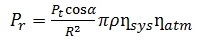 In terms of TLS systems, Eq. (7) can be written as:
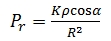 Where the term K = (PtDr2/4)ηSysηAtm in the original radar
range equation (Eq. (2)) is taken to be a constant. The power received,
Pr is taken to be equivalent to the recorded laser returned intensity.
The reflectance, incidence angle and range parameters are as defined
above. Eq. (8) is not an ideal physical model for all scenarios and this
is so because for most scanners, the intensity-distance correction tends
to be affected more by instrumental effects and these occur either for
measurements taken at shorter baselines or those taken at longer
baselines (Balduzzi et al., 2011).
3.2.1 Near-Distance Correction
Model
A number of researchers (e.g. Krooks et al., 2013) have reported that
the effects of the scanning distance and the incidence angle on the
intensity do not mix, implying that it is possible to solve these
effects independent of each other. According to Fang et al. (2015),
solving for the near-distance effects on the intensity involved
considering several parameters such as the Gaussian laser beam, the lens
formula, focusing of the lens and the computation of the detector’s
received power under the assumption that it is circular. In order to
avoid repetition, detailed information can be found in Fang et al.
(2015) and where it has been stated that for a coaxial laser scanner,
the near-distance effect can be described as the ratio of the input
laser signal that the detector captures between the limited range (R)
and unlimited range (∞) as shown in Eq. (9):
Where the term K = (PtDr2/4)ηSysηAtm in the original radar
range equation (Eq. (2)) is taken to be a constant. The power received,
Pr is taken to be equivalent to the recorded laser returned intensity.
The reflectance, incidence angle and range parameters are as defined
above. Eq. (8) is not an ideal physical model for all scenarios and this
is so because for most scanners, the intensity-distance correction tends
to be affected more by instrumental effects and these occur either for
measurements taken at shorter baselines or those taken at longer
baselines (Balduzzi et al., 2011).
3.2.1 Near-Distance Correction
Model
A number of researchers (e.g. Krooks et al., 2013) have reported that
the effects of the scanning distance and the incidence angle on the
intensity do not mix, implying that it is possible to solve these
effects independent of each other. According to Fang et al. (2015),
solving for the near-distance effects on the intensity involved
considering several parameters such as the Gaussian laser beam, the lens
formula, focusing of the lens and the computation of the detector’s
received power under the assumption that it is circular. In order to
avoid repetition, detailed information can be found in Fang et al.
(2015) and where it has been stated that for a coaxial laser scanner,
the near-distance effect can be described as the ratio of the input
laser signal that the detector captures between the limited range (R)
and unlimited range (∞) as shown in Eq. (9):
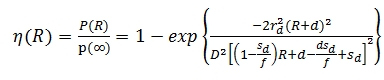 Where rd is the radius of the circular laser detector, d is the offset
between the measured range R and the object distance from the lens
plane, D is the diameter of the lens, Sd is the fixed distance of the
detector from the lens and f is the focal length. All of which are
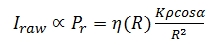
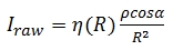
parameters of the laser scanner. Combining Eq. (9) with Eq. (8) and
taking into account the near-distance effect, the recorded raw intensity
(Iraw) value can be written as:
Where rd is the radius of the circular laser detector, d is the offset
between the measured range R and the object distance from the lens
plane, D is the diameter of the lens, Sd is the fixed distance of the
detector from the lens and f is the focal length. All of which are
parameters of the laser scanner. Combining Eq. (9) with Eq. (8) and
taking into account the near-distance effect, the recorded raw intensity
(Iraw) value can be written as:
 3.2.2 Oren–Nayar Reflectance
Model vis-à-vis Target Surface Roughness
An investigation which considered faceted surfaces in an attempt to
describe surface roughness was addressed in the Oren-Nayar reflectance
model (Oren and Nayar, 1994; Oren and Nayar, 1995) which makes a
prediction that a surface with facets returns more light in the
direction of the light source than a surface with Lambertian properties.
For a faceted surface, other than the global normal, each micro-facet
has its own normal and orientation. For some surfaces, each facet can
actually be a perfect diffuse reflector though this may not be so when
all the various facets are combined (Carrea et al., 2016). However, in a
case where the various facets are of the same size or smaller than the
wavelength, the behaviour tends to follow that of diffuse reflection.
But in a case where the facets are of a size that is almost as large as
the laser beam spot size, the returned intensity gets controlled by a
few facets.
In the Oren-Nayar reflectance model, an important parameter which models
the effect of a faceted surface on reflection is presented. This
parameter is the standard deviation of the slope angle of facets
(σslope) and it can be computed for different reflectivity surfaces. The
Oren–Nayar model is a Bidirectional Reflectance Distribution Function
(BRDF) since it models the reflectance with regards to both the
incidence and the reflection direction. The Oren–Nayar model is
expressed in the following form where the radiance is computed as
follows (Oren and Nayar, 1995):
3.2.2 Oren–Nayar Reflectance
Model vis-à-vis Target Surface Roughness
An investigation which considered faceted surfaces in an attempt to
describe surface roughness was addressed in the Oren-Nayar reflectance
model (Oren and Nayar, 1994; Oren and Nayar, 1995) which makes a
prediction that a surface with facets returns more light in the
direction of the light source than a surface with Lambertian properties.
For a faceted surface, other than the global normal, each micro-facet
has its own normal and orientation. For some surfaces, each facet can
actually be a perfect diffuse reflector though this may not be so when
all the various facets are combined (Carrea et al., 2016). However, in a
case where the various facets are of the same size or smaller than the
wavelength, the behaviour tends to follow that of diffuse reflection.
But in a case where the facets are of a size that is almost as large as
the laser beam spot size, the returned intensity gets controlled by a
few facets.
In the Oren-Nayar reflectance model, an important parameter which models
the effect of a faceted surface on reflection is presented. This
parameter is the standard deviation of the slope angle of facets
(σslope) and it can be computed for different reflectivity surfaces. The
Oren–Nayar model is a Bidirectional Reflectance Distribution Function
(BRDF) since it models the reflectance with regards to both the
incidence and the reflection direction. The Oren–Nayar model is
expressed in the following form where the radiance is computed as
follows (Oren and Nayar, 1995):
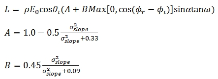 Where L is the radiance, E0 is the radiant flux received at normal
incidence angle in radians, ρ is the material reflectivity, α is the
incoming and ω the outgoing incidence angle, ϕr and ϕi are the reflected
and incident viewing azimuth angle in radians and σslope as the standard
deviation of the slope angle distribution in radians.
According to Carrea et al. (2016), the model Eq. (11) can be applied in
TLS systems where in terms of the configuration, the incidence and
reflected rays are coincident as expressed below:
Where L is the radiance, E0 is the radiant flux received at normal
incidence angle in radians, ρ is the material reflectivity, α is the
incoming and ω the outgoing incidence angle, ϕr and ϕi are the reflected
and incident viewing azimuth angle in radians and σslope as the standard
deviation of the slope angle distribution in radians.
According to Carrea et al. (2016), the model Eq. (11) can be applied in
TLS systems where in terms of the configuration, the incidence and
reflected rays are coincident as expressed below:
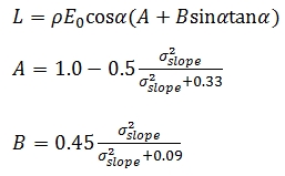
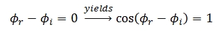 Therefore Eq. (11) which is a BRDF can be turned into a non-BRDF where α
the incoming incidence angle is equal to ω the outgoing incidence angle
and then rewritten as:
Therefore Eq. (11) which is a BRDF can be turned into a non-BRDF where α
the incoming incidence angle is equal to ω the outgoing incidence angle
and then rewritten as:
 3.2.3 Hybrid Intensity
Correction Model
Since Eq. (10) has K as a constant, it can be simplified and rewritten
as:
3.2.3 Hybrid Intensity
Correction Model
Since Eq. (10) has K as a constant, it can be simplified and rewritten
as:
 The corrected intensity (Icorr) value can be computed as follows
considering the near distance effects, material reflectivity, incidence
angle and range:
The corrected intensity (Icorr) value can be computed as follows
considering the near distance effects, material reflectivity, incidence
angle and range:
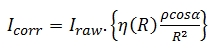 This intensity correction (Eq. (15)) can be used for perfect diffuse
scattering surfaces. However, for surfaces with micro-facets this
correction would not work well and so there is need to integrate the
standard deviation of the slope angle since each facet on the surface
has its own normal. Thus a hybrid intensity correction model that
considers near distance effects and also integrates the Oren-Nayar model
is proposed to improve the intensity correction.
This intensity correction (Eq. (15)) can be used for perfect diffuse
scattering surfaces. However, for surfaces with micro-facets this
correction would not work well and so there is need to integrate the
standard deviation of the slope angle since each facet on the surface
has its own normal. Thus a hybrid intensity correction model that
considers near distance effects and also integrates the Oren-Nayar model
is proposed to improve the intensity correction.
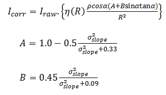 The standard deviation of the slope angle of facets (σslope) was
determined as in Carrea et al. (2016) and the following is an
explanation of the procedure. To obtain the optimal value for the slope
standard deviation (σslope), standardisation with respect to values
close to normal incidence was computed by using a sub-sample of points
that covered the area of the concrete block so as to reduce
computational intensity. Since the concrete blocks were fairly rough and
several points were scanned on the face on the block, it implies that
each point had its own incidence angle dependent on where the laser hit
on the block and the orientation of the normal at that position. This
being the case, an optimisation function was employed in order to
calculate the optimal value of σslope. Therefore, after the intensity
was corrected for near distance effects, it was then vital to compute
the optimal σslope value which would give a minimal variation of the
corrected intensity by taking into consideration the different incidence
angles. The optimisation function minimises the differences between the
mean corrected intensity values for the two intervals of the incidence
angle i.e. 0° to 10° and 0° to 45° by way of minimising to a single
variable on a fixed interval and so making it possible to obtain the
minimum of fσslope on a bounded interval [0, 1] as
written in Eq. (17) below:
The standard deviation of the slope angle of facets (σslope) was
determined as in Carrea et al. (2016) and the following is an
explanation of the procedure. To obtain the optimal value for the slope
standard deviation (σslope), standardisation with respect to values
close to normal incidence was computed by using a sub-sample of points
that covered the area of the concrete block so as to reduce
computational intensity. Since the concrete blocks were fairly rough and
several points were scanned on the face on the block, it implies that
each point had its own incidence angle dependent on where the laser hit
on the block and the orientation of the normal at that position. This
being the case, an optimisation function was employed in order to
calculate the optimal value of σslope. Therefore, after the intensity
was corrected for near distance effects, it was then vital to compute
the optimal σslope value which would give a minimal variation of the
corrected intensity by taking into consideration the different incidence
angles. The optimisation function minimises the differences between the
mean corrected intensity values for the two intervals of the incidence
angle i.e. 0° to 10° and 0° to 45° by way of minimising to a single
variable on a fixed interval and so making it possible to obtain the
minimum of fσslope on a bounded interval [0, 1] as
written in Eq. (17) below:
 The data processing and intensity correction method was implemented in
Matlab routines. The intensity value is dimensionless and for each
block, statistics such as intensity mean and standard deviation were
calculated. The average roughness (σslope) values for the blocks were
not so far away from 0° as values ranged from 1.15° to 2.58°. Concrete
reflectivity measurements were not taken due to non-availability of the
spectrometer which would measure reflectivity at a wavelength of 1500 nm
(which is the wavelength of the HDS7000 laser scanner used in this
study). However, we searched for documentation with concrete
reflectivity information at the desired wavelength and information was
found in Larsson et al. (2010). Based on this finding, the reflectance
of concrete is in the range between 0.300 to 0.400 (Fig. 4) and since
the concrete which was used in the study was gray and with some
roughness, it was a trial and error of reflectance values from 0.370 to
0.400.
The data processing and intensity correction method was implemented in
Matlab routines. The intensity value is dimensionless and for each
block, statistics such as intensity mean and standard deviation were
calculated. The average roughness (σslope) values for the blocks were
not so far away from 0° as values ranged from 1.15° to 2.58°. Concrete
reflectivity measurements were not taken due to non-availability of the
spectrometer which would measure reflectivity at a wavelength of 1500 nm
(which is the wavelength of the HDS7000 laser scanner used in this
study). However, we searched for documentation with concrete
reflectivity information at the desired wavelength and information was
found in Larsson et al. (2010). Based on this finding, the reflectance
of concrete is in the range between 0.300 to 0.400 (Fig. 4) and since
the concrete which was used in the study was gray and with some
roughness, it was a trial and error of reflectance values from 0.370 to
0.400.
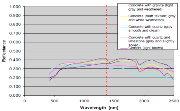
Fig. 4: Reflectivity spectrum of concrete and cement (Larsson et al.,
2010)
4. RESULTS AND ANALYSIS
4.1 Intensity Standard Deviation and Distribution of
Data
The data acquired was analyzed to study for each block the relation
between intensity standard deviation and intensity mean as was scanned
at the five various incidence angles labelled A to E (see measurement
setup in Fig. 3) and results are as shown in Fig. 5 below.
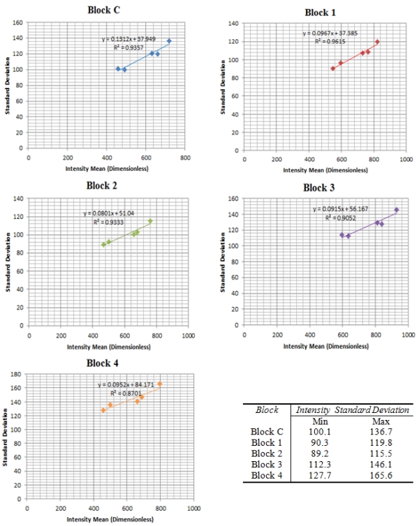 Fig. 5: Intensity
standard deviation against intensity.
Apparently, the standard deviation grows with the intensity mean for
each block and this is verified in Fig. 5. Regardless of the scanning
incidence angles which were 45°, 25°, 0°, -25° and -45°, the strength of
the linear relationship between the two variables in Fig. 5 is strong as
can be seen by the values of the coefficient of determination for each
block. The minimal variation of the coefficient of determination of the
blocks is due to the fact that their surfaces were not totally
homogenous because the concrete aggregate cannot be uniformly
distributed in all blocks although the same mix design was used.
The distribution of the intensity data for the blocks scanned at various
incidence angles was as assessed and taking Block C as an example, the
results are as shown in Fig. 6.
Fig. 6: Intensity data distribution at various incidence angles
With reference to Fig. 6, two statistical parameters i.e. intensity mean
and standard deviations were further investigated in exploratory data
analysis of the intensity return at the various incidence angles. The
data is normally distributed in all cases and as expected. In terms of
the frequency, although the maximum count of 1800 was achievable at all
incidence angles, the overall maximum mean intensity return was higher
at normal angle of incidence where the point density is also high due to
the nature of static TLS. Furthermore, as already pointed out in Fig. 5,
the standard deviation grows with the intensity mean in Fig. 6.
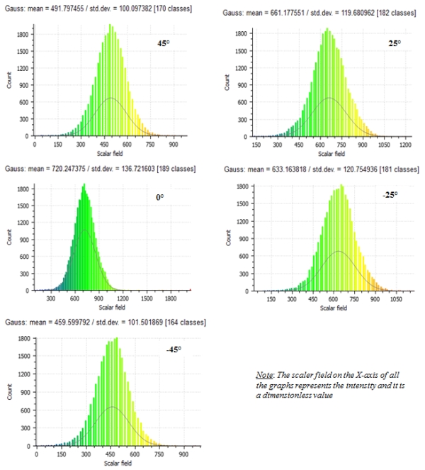
Fig. 6: Intensity data distribution at various incidence angles
4.2 Intensity and Incidence Angle (Before Correction)
The blocks were scanned at various incidence angles with the distance at
each scanning station held fixed. Fig. 7 and 8 show the resultant
relationship between uncorrected intensity for all the blocks and the
scanning angle of incidence.
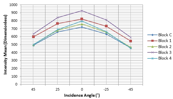 Fig. 7: Uncorrected intensity against incidence angle
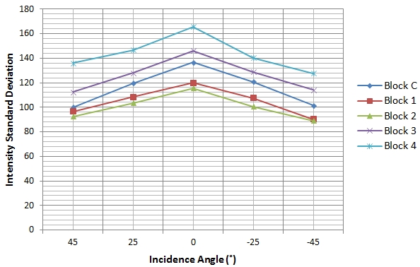 Fig. 8: Uncorrected intensity standard deviation against incidence angle
The incidence angle effect in both Fig. 7 and 8 is visible and all
blocks show the trend where the intensity decreases as the incidence
angle increases and this is true theoretically, based on the radar range
equation. As reported in theory, it can be seen that the closer the
laser beam incidence angle is to 0° the more the returned intensity.
Generally, higher incidence angles lead to a reduction in the amount of
returned intensity and this becomes more pronounced when incidence
angles are greater than 20° (Krooks et al., 2013) and for a Lambertian
reflecting surface, the returned intensity has been predicted to
decrease with the cosine of the incidence angle in accordance with
Lambert’s cosine law (Eq. (18)):
 Although Eq. (18) is a simplified mathematical law and the light
scattering behaviour of all natural surfaces is not Lambertian, the
incidence angle dependence for many surfaces is approximated to follow
the cos α relation (Kaasalainen et al., 2009b) as exemplified above.
4.3 Intensity and Distance (Before Correction)
The assessment of the distance effects on the intensity involved keeping
fixed the various incidence angles and only varying the distances when
scanning the concrete blocks. The relationships between the uncorrected
intensity and the distance are as shown in Fig. 9.
Although Eq. (18) is a simplified mathematical law and the light
scattering behaviour of all natural surfaces is not Lambertian, the
incidence angle dependence for many surfaces is approximated to follow
the cos α relation (Kaasalainen et al., 2009b) as exemplified above.
4.3 Intensity and Distance (Before Correction)
The assessment of the distance effects on the intensity involved keeping
fixed the various incidence angles and only varying the distances when
scanning the concrete blocks. The relationships between the uncorrected
intensity and the distance are as shown in Fig. 9.
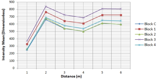 Fig. 9: Uncorrected intensity against distance
The distance effects on the intensity can be seen since in theory, the
returned intensity is expected to decrease with an increase in distance.
The plausible reason for the unexpected results was atributed to the
instrumental effects at short scanning distances and such results have
also been reported by other researchers (e.g. Kaasalainen et al., 2011)
although different scanners were used. Furthermore, in the same vein,
Höfle (2014) states that past studies on TLS radiometric correction have
clearly shown that the range dependence of TLS amplitude and intensity
does not entirely follow the 1/R2 law of the radar equation as mostly
valid for ALS, in particular at near distance of for instance less than
15 m. The reasons can be detector effects (e.g., brightness reducer,
amplification, and gain control or receiver optics (defocusing and
incomplete overlap of beam and receiver field of view). However, most
manufacturers do not provide enough insight into developing a
model-driven correction of these effects.
4.4 Intensity and Cosine Law Prediction vis-à-vis
Incidence Angle
The theoretical contribution of the incidence angle to the deterioration
of the returned intensity is plotted in Fig. 10 and it follows Eq. (18).
The function 1/cos(α) was also applied and it gave the same result in
Fig. 10 and according to Yan and Shaker (2014), this is why the cosine
of the incidence angle is commonly taken to be indirectly proportional
to the corrected intensity (or spectral reflectance) in the correction
process.
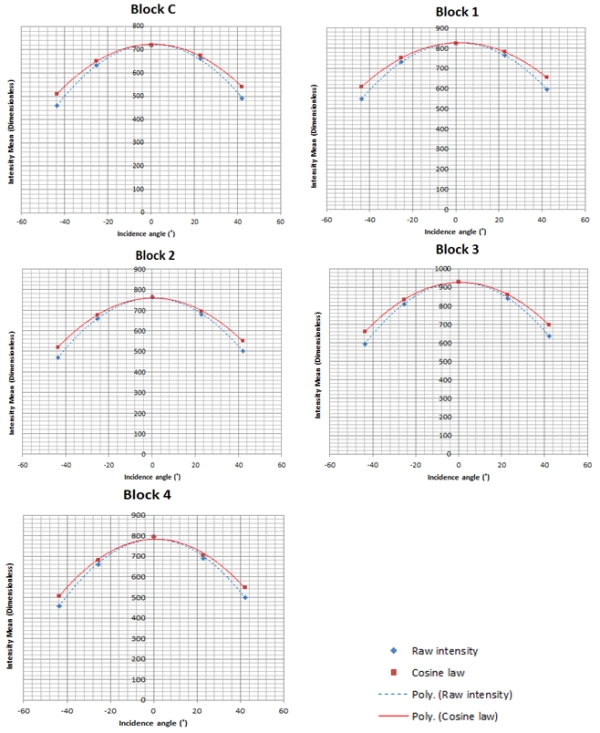 Fig. 10: Raw intensity and cosine law against incidence angle
The relationship between the intensity and the incidence angle as well
as Lambert’s cosine law is shown in Fig. 10. A close correlation between
the raw intensity and that with the cosine law is evident though a
constant and an offset of the cosine of the incidence angle may have to
be added for more accurate results as suggested in Kaasalainen et al.
(2011). However, Lambert’s cosine law still provides a good
approximation of the incidence angle effects, especially up to about 20°
of incidence (Kaasalainen et al., 2009b). Lambert’s cosine law can
provide a satisfactory estimation of light absorption modelling for
rough surfaces in both active and near-infrared spectral domains, thus,
it is widely employed in existing intensity correction applications.
However, Lambert’s cosine law is insufficient to correct the incidence
angle effect for surfaces with increasing irregularity because these
surfaces do not exactly follow the Lambertian scattering law. The
incidence angle is related to target scattering properties, surface
structure and scanning geometry. The interpretation of the incidence
angle effect in terms of target surface properties is a complicated task
(Tan and Cheng, 2016). However, Lambert’s cosine law has been
successfully applied in some studies to correct the intensity for
incidence angle effects. For instance, in Pfeifer et al. (2007) an
experiment is reported with an Optech ILRIS3D laser scanner, where one
target with near Lambertian scattering characteristics scanned at a
distance close to 7m was observed at different angles. The intensity was
corrected using the cosine correction and a linear amplification model.
To visualize the effect of the cosine law on the intensity values in
overall scale, the average difference between the raw and cosine
predicted intensity data points was plotted as shown in Fig. 11(a) for
Block C as an example. Fig. 11(b) shows the raw intensity of Block C and
the error bars indicate the average standard deviation.
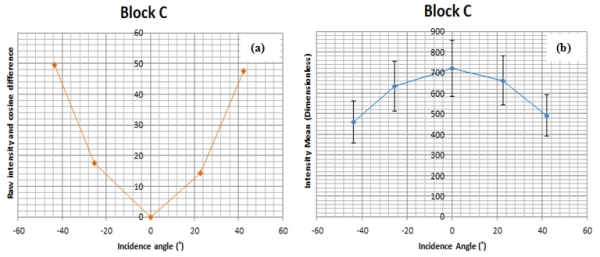 Fig. 11: Difference between raw intensity and cosine law against
incidence angle
Compared to the error range of the intensity for Block C in Fig. 11(b),
the difference between the raw intensity and that with the cosine law is
still quite minimal, which in percentage terms ranges from 0% at normal
incidence angle to about 11% at 45°. This means that the accuracy of the
cosine law is sufficient to predict the reflectance at this level of
accuracy but may have limitations at higher angles of incidence as
already pointed out above. However, the improved intensity correction
method did not relay on the cosine law for incidence angle correction
since it is insufficient to consider target surface characteristics, and
more so its limitations beyond 20° of incidence angle.
4.5 Improved Intensity Correction Method
The procedural steps for the improved intensity correction method
involve, first correcting intensity data for near-distance effects which
are evident in Fig. 9 by applying the near-distance correction method
presented above and after that the incidence angle and distance effects
on the intensity can be solved separately since they do not mix.
According to Fang et al. (2015), in a study where the Z+F Imager 5006i
laser scanner was used, the parameters in Eq. (9) have a physical basis
and that the derived parameters in Table 2 were estimated in accordance
with observed values such as the receiver’s diameter and the detector’s
distance from the lens plane by iterative curve fitting using a
nonlinear least squares method and robust Gauss-Newton algorithm.
However, the values of the parameters differ for the various laser
scanners and so each laser scanner needs to be studied.
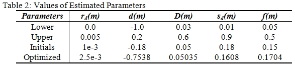 Although the estimated parameters in Table 2 were obtained using the Z+F
Imager 5006i laser scanner, the parameters were tested for the HDS7000
laser scanner with success since the two instruments are coaxial and
basically identical in terms of their physical characteristics as
designed by the manufacturer. Fig. 12 below shows the results after
applying the near-distance correction and it can be seen that the
correction is valid for distances from 2m and greater since all the
other scanning distances investigated follow the theoretical range
squared inverse law in relation to the returned intensity and the
measured distances. As already alluded to above, instrumental effects
such as near-distance reducers (which are meant to avoid over-exposure
of the sensor) are known to have an influence on the returned intensity
and this actually makes the laser range equation to be inapplicable at
all distances as a physical model for intensity correction.
Although the estimated parameters in Table 2 were obtained using the Z+F
Imager 5006i laser scanner, the parameters were tested for the HDS7000
laser scanner with success since the two instruments are coaxial and
basically identical in terms of their physical characteristics as
designed by the manufacturer. Fig. 12 below shows the results after
applying the near-distance correction and it can be seen that the
correction is valid for distances from 2m and greater since all the
other scanning distances investigated follow the theoretical range
squared inverse law in relation to the returned intensity and the
measured distances. As already alluded to above, instrumental effects
such as near-distance reducers (which are meant to avoid over-exposure
of the sensor) are known to have an influence on the returned intensity
and this actually makes the laser range equation to be inapplicable at
all distances as a physical model for intensity correction.
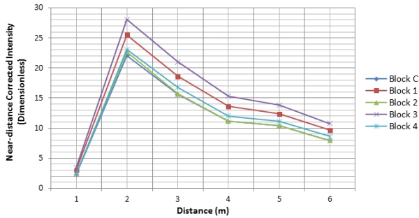 Fig. 12: Near-distance corrected intensity against distance
4.5.1 Intensity and Distance
(After Correction)
Fig. 13 below shows the results of the relationship of intensity against
distance after applying correction on the intensity data. With the
exception of 1m, the correction is valid from 2m and all the other
distances that the concrete was scanned from.
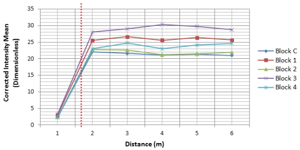 Fig. 13: Corrected intensity against Distance
4.5.2 Intensity and Incidence
Angle (After Correction)
The relationship of the corrected intensity against incidence angle is
as shown in Fig. 14. It can be observed that for all the angles of
incidence that were investigated, the intensity correction method is
valid. The incidence angle effect on the intensity decreased as the
graphs for all the blocks tend to straighten cross the whole range of
the incidence angles.
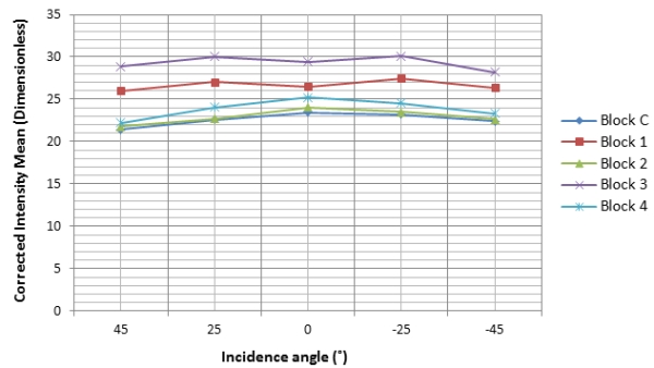 Fig. 14: Corrected intensity against incidence angle
Although the incidence angle effects appear to have significantly
reduced in Fig. 14, the dominance of the reflectance for each block on
the incidence angle behaviour can be seen and this could be because the
blocks were not completely the same.
5. DISCUSSION AND CONCLUSION
The effects of the distance and incidence angle on the intensity of
concrete specimens have been analysed by looking at the relationship of
each with the intensity and they were found to be independent as also
reported by some past researchers and this makes it possible to correct
both by using different models that are independent of the measurement.
Results of the uncorrected intensity and distance relationship have
shown that intensity measurements from the HDS7000 scanner at near
distances have instrumental effects and several other researchers as
mentioned in the reviewed material have reported a similar finding even
though different types scanners were used. The distance and incidence
angle effects for the HDS7000 concrete intensity data were corrected
using the improved method and this method has shown the potential to
correct the intensity at scanning distances from 2m and greater. The
correction of intensity for near distance effects is important for
studies that require measurements to be taken at shorter baselines. The
raw intensity in relation to that with the cosine law prediction did
show a close relationship indicating that the cosine law provides a good
approximation of the incidence angle effects and the more reason it is
used in intensity correction schemes. However, Reshetyuk (2006) observed
that the intensity return decreased with an increase in angle of
incidence through experiments carried out using the HDS3000 scanner
although the scanned target (a wall) was not Lambertian. It has been
reported in some studies that even when the raw intensity may appear to
follow the cosine law prediction, there is no guarantee that the
Lambert’s cosine law would correct the intensity data for incidence
angle effects as for instance pointed out in Tan and Cheng (2016) where
a FARO Focus3D 120 scanner was used and a differerent intensity
correction method was actually applied. Furthermore, they have stated
that the incidence angle is related to target scattering properties,
surface structure and scanning geometry and that the interpretation of
the incidence angle effect in terms of target surface properties is a
complicated task. Surface roughness of the scanned target is also a
factor that can influence the returned intensity and the concrete that
was used in this study had roughness ranging from millimeters to a few
centimeters. Athough the magnitude of concrete roughness may seem to be
small, it had an influence though minimal on the intensity correction.
An improved intensity correction method such as the one presented could
be potentially beneficial in several applications such as change
detection, material classification and segmentation.
The following conclusions have been drawn from this study and in
relation to the wider context of the subject in past research work:
- An intensity correction model that
considers near distance effects and also integrates the Oren-Nayar model
so as to account for target roughness has been presented. The results
achieved in the study are promising though more work still needs to be
done as pointed out in the section for suggested areas of further
research.
- Several researchers have investigated
the subject of TLS intensity correction as shown in the material that
has been reviewed and it seems that a standard intensity correction
method for all the different types of scanners does not exist yet.
However, in Tan and Cheng (2015) it is argued that the proposed
correction model can be applied to correct intensity data acquired with
any scanner. This calls for more scanners to be tested.
- The fact that different intensity
correction methods have so far been proposed and some of which are
complex, implies that the intensity fluctuations for any type of scanner
may not be easily modelled. Furthermore, there is need to know what each
scanner records, whether it’s the intensity or the amplitude.
- Instrumental effects on the returned
intensity vary depending on the type of scanner and the manufacturer.
However, for most scanners, the intensity-distance correction tend to be
affected more by instrumental effects and these occur either for
measurements taken at shorter baselines or those taken at longer
baselines. This implies that the performance of each scanner has to be
properly studied.
SUGGESTIONS OF FUTURE RESEARCH
- The subject of TLS intensity correction
is still an open area of investigation and this research is still
on-going and future research will consider using the spectrometer and
the VNIR hyperspectral camera (which operate at the wavelength of the
TLS) for extracting spectral charateristics of the concrete specimens.
- The concrete blocks that were used in
this study were not significantly rough and so future research work will
test the method to correct intensity data of scanned objects with
significant rough surfaces and with measurements taken at close range as
was done in this study. Furthermore, correction for the incidence angle
effects will need to be compared to that based on the linear combination
of the Lambertian and Beckmann law.
- Most TLS intensity correction methods
that have been proposed in some past research work have often used
targets of known reflectivity such as spectralons for calibration
purposes to obtain the device constants or to determine the effects of
near-distance reducers. There is need to test some of the correction
methods with several natural targets.
ACKNOWLEDGEMENTS
The Authors express their gratitude to The University of Nottingham
Ningbo China for the financial support and massive contribution in terms
of the research facilities which made this study to be undertaken and
many thanks to the FIG Foundation for co-funding the work through the
scholarship which was awarded to the PhD student.
REFERENCES
- Anttila, K, Kasalainen, S, Krooks, A, Kaartinen, H, Kukko, A, Manninen,
T, Lahtinen, P and Siljamo, N (2011) Radiometric Calibration of TLS
Intensity: Application to Snow Cover Change Detection. International
Archives of the Photogrammetry, Remote Sensing and Spatial Information
Sciences, 38 (5/W12), 175-179.
- Balduzzi, M.A.F, Van der Zande, D, Stuckens, J, Verstraeten, W.W and
Coppin, P. (2011) The properties of terrestrial laser system intensity
for measuring leaf geometries: A case study with conference pear trees
(Pyrus Communis). Sensors, 11, 1657-1681.
- Blaskow, R and Schneider, D (2014) Analysis and Correction of the
Dependency between Laser Scanner Intensity Values and Range. The
International Archives of the Photogrammetry, Remote Sensing and Spatial
Information Sciences, Volume XL-5, 2014. ISPRS Technical Commission V
Symposium, 23 – 25 June 2014, Riva del Garda, Italy.
- Carrea, D., Abellan, A., Humair, F., Matasci, B., Derron, M. and
Jaboyedoff, M. (2016) Correction of terrestrial LiDAR intensity channel
using Oren–Nayar reflectance model: An application to lithological
differentiation. ISPRS Journal of Photogrammetry and Remote Sensing,
113, 17-29.
- Fang, W, Huang, X, Zhang, F and Li, D (2015) Intensity Correction
of Terrestrial Laser Scanning Data by Estimating Laser Transmission
Function. IEEE Transactions on Geoscience and Remote Sensing, 53, (2)
942-951
- Franceschi, M., Teza, G., Preto, N., Pesci, A., Galgrao, A. and Girardi,
S. (2009) Discrimination between marls and limestones using intensity
data from terrestrial laser scanner. ISPRS Journal of Photogrammetry and
Remote Sensing, 64, 522–528.
- Habib, A, Kersting, A, Shaker, A and Yan, W.Y. (2011) Geometric
Calibration and Radiometric Correction of Lidar data and their Impact on
the Quality of Derived Products, Sensors, 11 (9) 9069-9097.
- Höfle, B. (2014) Radiometric Correction of Terrestrial LiDAR Point Cloud
Data for Individual Maize Plant Detection. IEEE Geoscience and Remote
Sensing Letters, 11(1) 94-98.
- Höfle B and Pfeifer N. (2007) Correction of laser scanning intensity
data: Data and model-driven approaches. ISPRS Journal of Photogrammetry
and Remote Sensing. 62 (6) 415-433.
- Jelalian, A. V (1992) Laser Radar Systems, Artec House, Norwood, MA USA.
- Kaasalainen, S, Jaakkola, A, Kaasalainen, M, Krooks, A and Kukko, A
(2011) Analysis of Incidence Angle and Distance Effects on Terrestrial
Laser Scanner Intensity: Search for Correction Methods. Remote Sensing,
3, 2207-2221.
- Kaasalainen, S, Krooks, A, Kukko, A and Kaartinen, H. (2009a)
Radiometric calibration of terrestrial laser scanners with external
reference targets. Remote Sensing, 1 (3) 144-158.
- Kaasalainen, S, Vain, A, Krooks, A and Kukko, A (2009b) Topographic and
distance effects in laser scanner intensity correction, in: Laser
scanning 2009, IAPRS, pp. 219–223.
- Kaasalainen S, Kukko A, Lindroos T, Litkey P, Kaartinen H., Hyyppä J,
Ahokas E. (2008) Brightness Measurements and Calibration with Airborne
and Terrestrial Laser Scanners. IEEE Transactions on Geoscience and
Remote Sensing. 46 (2) 528–534.
- Krooks, A, Kaasalainen S, Hakala T, and Nevalainen, O (2013) correction
of intensity incidence angle effect in terrestrial laser scanning ISPRS
annals of the photogrammetry, remote sensing and spatial information
sciences, volume II-5/w2, ISPRS workshop laser scanning 2013, 11-13
November 2013, Antalya, Turkey.
- Larsson, H., Hallberg, T., Elmqvist, M., Gustafsson, F. (2010)
Background and target analysis from a Ladar perspective - Reflectance
and penetration properties. FOI-R-- 3014 –SE ISSN 1650-1942.
- Leica Geosystems (2012) HDS7000 User Manual (on-line)
http://hds.leica-geosystems.com, accessed on 14th July 2014.
- Oren, M. and Nayar, S. K. (1994). Seeing beyond Lambert's law.
Computer Vision — ECCV '94: Third European Conference on Computer Vision
Stockholm, Sweden, May 2–6 1994 Proceedings, Volume II. J.-O. Eklundh.
Berlin, Heidelberg, Springer Berlin Heidelberg: 269-280.
- Oren, M. and Nayar, S. K. (1995) Generalization of the Lambertian model
and implications for machine vision. International Journal of Computer
Vision, 14(3), 227-251.
- Penasa, L, Franceschi, M, Preto, N, Teza, G and Polito, V (2014)
Integration of intensity textures and local geometry descriptors from
Terrestrial Laser Scanning to map chert in outcrops. ISPRS Journal of
Photogrammetry and Remote Sensing, 93, 88-97.
- Pfeifer, N, Dorninger, P, Haring, A. and Fan, H (2007) Investigating
terrestrial laser scanning intensity data: quality and functional
relations. Proceedings of VIII Conference on Optical 3D Measurement
Techniques, ETH Zurich, Switzerland (2007), pp. 328–337
- Reshetyuk, (2006) Investigation and Calibration of Pulsed Time-of-Flight
Terrestrial Laser Scanners. Ph.D. thesis, Royal Institute of Technology
(KTH), Division of Geodesy, Stockholm, Sweden.
- Shan, J and Toth, C.K. (2009) Topographic Laser Ranging and Scanning:
Principles and Processing, CRC Press.
- Soudarissanane, S., Lindenbergh, R., Menenti, M. and Teunissen, P.
(2009) Incidence Angle Influence on the Quality of Terrestrial Laser
Scanning Points. International Archives of the Photogrammetry, Remote
Sensing and Spatial Information Sciences, 38 (3/W8), 183-188.
- Soudarissanane, S, Lindenbergh, R, Menenti, M. and Teunissen P. (2011)
Scanning Geometry: Influencing Factor on the Quality of Terrestrial
Laser Scanning Points. ISPRS Journal of Photogrammetry and Remote
Sensing, 66 (4) 389-399.
- Tan, K. and Cheng, X. (2015) Intensity data correction based on
incidence angle and distance for terrestrial laser scanner. Journal of
Applied Remote Sensing, 9, 094094:1–094094:22.
- Tan, K. and Cheng, X. (2016) Correction of Incidence Angle and Distance
Effects on TLS Intensity Data Based on Reference Targets. Remote
Sensing, 8 (3) 251.
- Tan, K., Cheng, X., Ding, X. and Zhang, Q. (2016) Intensity data
correction for the distance effect in terrestrial laser scanners. IEEE
Journal of Selected Topics in Applied Earth Observations and Remote
Sensing, 9, 304–312
- Vain, A and Kaasalainen, S. (2011) Correcting Airborne Laser Scanning
Intensity Data, Laser Scanning, Theory and Applications, Prof.
Chau-Chang Wang (Ed.), ISBN: 978-953-307-205-0, InTech, DOI:
10.5772/15026. Available from:
http://www.intechopen.com/books/laser-scanning-theory-and-applications/correcting-airborne-laser-scanning-intensity-data
- Yan, W.Y and Shaker, A. (2014) Radiometric Correction and Normalization
of Airborne LiDAR Intensity Data for Improving Land-Cover Classification,
IEEE Transactions on Geoscience and Remote Sensing, 52 (12) 7658-7673.
- Zhu, X., T. Wang, T., Darvishzadeh, R., Skidmore, A. K. and Niemann, K.
(2015) 3D leaf water content mapping using terrestrial laser scanner
backscatter intensity with radiometric correction. ISPRS Journal of
Photogrammetry and Remote Sensing, 110, 14-23.
BIOGRAPHICAL NOTES
Wallace Mukupa is a post graduate research student in the Department of
Civil Engineering at The University of Nottingham, Ningbo, China. He is
currently pursuing a PhD in Engineering Surveying of civil structures.
Gethin W. Roberts is a Reader in Geospatial Engineering at The
University of Nottingham, United Kingdom. He is the UN Delegate for the
FIG through the Chartered Institution of Civil Engineering Surveyors. He
is a past chairman of FIG Commission 6.
Craig M. Hancock is an Assistant Professor in Geospatial Engineering at
The University of Nottingham, Ningbo, China. He is also involved with
the International Federation of Surveyors (FIG) and has been a Vice
Chair for communications on Commission 6 (Engineering Surveys) from 2010
– 2013.
Khalil Al-Manasir is an Assistant Professor in Geospatial Engineering at
Middle East University, Amman, Jordan. He has worked at The University
of Nottingham, Ningbo, China before as Assistant Professor.
CONTACT
Wallace Mukupa
The University of Nottingham, Ningbo, China.
Faculty of Science and Engineering
Department of Civil Engineering
199 Taikang East Road
Ningbo 315100
CHINA
Email: wallace.mukupa@nottingham.edu.cn
|


