Article of the Month -
May 2013
|
Revisiting the Interaction between the Nigerian Residential Property
Market and the Macroeconomy
Ismail OJETUNDE, Nigeria
1) This paper is a Nigerian
Peer Review paper, which was presented at FIG Working Week 2013, 6-10
May, in Abuja, Nigeria. Like last month article, this paper highlights
one of the challenges Nigerian surveyors are dealing with, namely the
Nigerian property market. At the conference many papers highlighted the
current challenges Nigerians surveyors are faced with. You can find the
papers
here.
Key words: Macroeconomy, property, property market,
residential, rents.
SUMMARY
The study of residential price dynamics and macro economic
developments are important for virile economic and social policies
formulation at both local and national scales. This paper revisits the
interaction between the Nigerian macroeconomy and the operation of its
residential property market using econometric analysis. By employing a
larger sample and different data analysis approaches (pairwise
correlations, cointegration, granger causality and vector
autoregression) the objective is to provide further evidence on the
extent to which the property market is integrated or linked to
macroeconomy. Evidence suggests that macroeconomic variables (real gross
domestic product, inflation, exchange and interest rates) have long term
relationship with residential property rents in Nigeria. The results of
the granger causality shows that both exchange and interest rates have
useful information for predicting residential property rents over and
above the past values of other macroeconomic variables. Aside, the
result of the variance decomposition within the vector autoregressive
model further confirmed that real GDP and Exchange rate combined
forecast 31.4% of the variance in residential property rents. This study
concludes that the response of the residential property market to
macroeconomic shocks of interest rate, real GDP, and exchange rate
implies a relatively slow adjustment of the property market to the ever
changing macroeconomic events in Nigeria making long run equilibrium
elusive. These findings are significant for the continued development of
the Nigerian property market which is fraught with poor market
information.
1. INTRODUCTION
Residential property is a dynamic commodity characterized by
structural durability, spatial immobility and its physically modifiable
nature. As a consumption and investment commodity, residential property
exerts profound influence on the socio-economic and psychological
well-being of individuals, households and socio-ethnic groups. Since
residential property constitutes the bulk of any country’s tangible
capital, the study of residential price dynamics and macro economic
developments are important for economic and social policies formulation
on both local and national scales. Numerous theoretical and econometric
studies have however investigated the relationship between residential
price (which has remained a significant feature of most markets for
housing services in the world) and the economy (for example, see Barras
and Ferguson, 1985, 1987a & 1987b; Hekman, 1985; Kling and McCue, 1987&
1991; DiPasquale and Wheaton, 1996). Aside investigating the link
between property and the wider economy, a point of convergence in these
previous literature, is the existence of interaction and interdependency
between property and the economy. For instance, during periods of
macroeconomic stability, cycles in property tend to be endogenous
(caused by disequilibria in the sector) and are relatively subdued and
in periods of macroeconomic instability, property cycles tend to be
exogenous (caused by various conditions in the macroeconomy) and
sometimes feature exceptional fluctuations (Dehesh and Pugh, 1995
p.2581). Although this cause and feedback mechanisms described by Dehesh
and Pugh (1995)is a feature of most market based system, the focal point
of this research however is not on endogenous influences, but rather the
nexus between real estate and exogenous influences of the economy.
Earlier studies of this nature provided evidence on the link between
property and the exogenous factors of the economy but have been
considerably skewed to only the United kingdom and United States (McCue
and Kling, 1994; Brooks and Tsolasco, 1999; Ling and Naranjo, 2003) with
both countries having well integrated and transparent property markets.
In developing countries, such evidence is limited to India (Joshi, 2006;
Vishwakarma and French, 2010). In Nigeria, recent study by Ojetunde et
al. (2011) has empirically discountenance the assumption that the
residential property market in Nigeria is not coupled or linked with the
economy. This research revisit the interaction between the economy and
the operation of the residential property market by extending the study
period (between 1984 and 2011) and improving on the data analysis
approaches in Ojetunde et al. (2011) study. Unlike studies in developed
economies which employed data on paper-backed securities, this study
explore the use of nominal rents from direct property investment in the
absence of property returns from the Nigerian Stock Market.
2. THE OPERATION OF THE RESIDENTIAL PROPERTY MARKET AND THE
ECONOMY: A REVIEW
Unlike other highly durable goods, the market for property and by
extension, the operation of residential property presents a somewhat
peculiar complexity as it comprises three (3) independent but connected
markets linked to the economy. Fig.1 provides for a simple residential
property model and link it with other exogenous systems (local and
national economies and the capital markets). To start with, the model
shows three important components (space, asset and development markets)
which on their own represent market arenas where trade take place and
prices are determined through demand and supply interplay ( Keogh 1994;
Fischer 1999 and Geltner et al., 2007).
The space market involves the interaction of the demand by
residential property users with the current stock of space made
available by the landlords. It is this result of demand-supply
interaction which predicts the pattern of rents and the level of
occupancy with vacancy clearing the market. Within the space market, the
demand for residential space is aptly affected by the national and local
economies. A growth in real wages for example may encourage new
households’ formation and hence an increase in demand for residential
physical space. For instance, property rights can be packaged in the
short run in form of use rights to property users in return for
residential rents (use values).
In the asset market, Viezer, (1999) concludes that the rent
determined in the space market is central in determining the demand for
real estate assets because this cash flow in form of rents interacts
with the cap rates required by investors, with the end product being the
property market/ capital values.
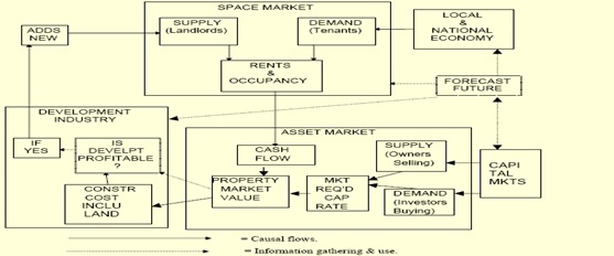
Fig.1: A Model of Residential Property Market: Interaction of the Space,
Asset and the
Development Markets with other Exogenous Systems. Source: Geltner et
al.,(2007).
As such what investors are really buying is the discounted present
value of asset’s expected income flow. The cap rates which investors
require in sealing real estate transactions in the asset market are
affected by opportunity cost of capital (since the desirability of
buying and selling real estate must be considered within a wide spectrum
of other investment opportunities operating within the capital markets),
growth expectation of future rents and investors perception of risk
associated with real estate investment vis-à-vis other investment
outlets in the capital markets (Ling and Archer, 1997b and Geltner et
al., 2007).
On one hand, clear independency however exists between space (use)
and asset markets with respect to right to use space (user rights) as
different from the right to hold a purely financial investment interest
in property (investor rights). On the other hand, connectivity is
evident as the use and investment rights subsisting in a property
ownership (for instance in an unencumbered freehold interest) is
mediated through the development market to meet changing market
requirements of users and investors. It is these market changes in users
and investors requirements which stimulate development activity and
development in turns supplies new user and investors rights into the
market (Keogh, 1994). For example, development would only occur insofar
as property rent can offset the long run marginal cost of a property
(Geltner et al., 2007). It is this singular condition which ensures that
the development market employ physical and financial resources to
construct new built space as well as refurbishment, rehabilitation or
conversion of existing buildings. The role of development therefore
comes to bear in differing ways: An economy in recession needs existing
built space so as to continue to function. Conversely, structural
changes in form of modifying existing dwellings (through refurbishment
and conversion) and new construction of dwellings (resulting from
outward expansion on undeveloped land) is necessary due to economic
growth or structural shifts in the economy.
Aside the foregoing simple property market model, numerous empirical
studies by Barras, (1983); Barras and Ferguson, (1987a, 1987b) and
Barras, (1994) have shown how building boom is triggered through the
combinations of conditions in the real economy, credit economy and
property market. The focal point of these studies is the derivation of a
theoretical framework which has been tested using time-series modelling
techniques to uncover the dynamics and operations within the property
market. Exploring this theme with minor variant, Dehesh and Pugh (1995,
p.2583) have also show considerable evidence that cycles in property has
deep cause-consequence interdependency on the financial and credit
cycles even at a global scale. They further argue that such structural
change resulting from changes in the financial sector requirements may
occur contemporaneously with and interact with the fluctuations in both
the macroeconomy and the credit markets, thereby heightening inflation,
causing financial collapse and leading to recession in the property
sectors.
Previous studies linking property to the economy over time, however,
fall principally into two distinct categories: those that centre
explicitly on property- backed securities such as real estate investment
trusts (Hartzell et al., 1987; Chan et al., 1990; McCue and Kling, 1994;
Brooks and Tsolacos, 1999; Ling and Naranjo, 1997; Ling and Naranjo,
2003) as against those on direct property market variables, as diverse
as construction series and rents ( Kling and McCue, 1987 ; Kling and
McCue, 1991 ; Giussani, et al., 1992). Table 1 summarizes previous
empirical research linking property with the economy. These empirical
investigations are preponderant in the USA with most employing vector
autoregressive framework as their methodology and few using regression
analysis.
Within the first category, Chan et al. (1990) for instance examine
the connection between some pre-specified macroeconomic variables and
real estate returns from the stock market using regression analysis.
They find that changes in risk, unexpected inflation and term structure
are significant predictors; while changes in industrial production and
expected inflation have no significant influence on real estate returns.
McCue and Kling (1994) however extend the examination of the link
between property and the economy in another direction. They treat real
estate returns as a residual by controlling for the covariance between
equity REIT returns and the overall stock market resulting from industry
effects. In their analysis, the authors employ vector autoregressive
model to test the relationships between this real estate residual and
macroeconomic variables and conclude that macroeconomic variables
account for 60% variance in real estate returns.
Brooks and Tsolacos (1999) take a similar approach to McCue and Kling
(1994) study by also removing the impact of the general stock market on
equity REIT series but using UK dataset. They suggest that unexpected
inflation and term structure have a contemporaneous rather than a lagged
effect on property returns. The absence of lagged effect however implies
that changes in unexpected inflation and term structure are quickly
incorporated into property returns. The authors further contend that
property returns are explained by own lagged values: current property
returns may have predictive power for future property returns. They
hypothesise that this own lagged effect is partly due to the fact that
property returns may reflect property market influences (rents, yield
and vacancy rates) rather than macroeconomic variables and partly
because macroeconomic and property data are not in a direct measurable
form.
A departure from the above categorization is the studies by Kling and
McCue (1987) and Kling and McCue (1991) who focus on property market
indicator. They advocate the use of construction series from direct real
estate investment and employ vector autoregressions to model industrial
and office construction cycles. They find that macroeconomic variables
influence real estate series indirectly through other macroeconomic
variables. The authors also show that adjustment to macroeconomic shocks
take place with a lag, resulting from the existence of long production
period between new construction starts and completions.
Giussani et al. (1992) also examine the relationship between changes
in commercial rental values and fluctuations in economy activity using a
predictive model. They analyse monthly data from 1983 to 1991 from
Europe and find that real Gross Domestic Product (GDP) is the most
significant explanatory variable for rental values. This result is
consistent with those reported in Hetherington (1988) and Keogh (1994)
that GDP is a determinant of rents, to the extent that rents are closely
correlated with the business cycle.
Table 1. Classification of Studies Linking Property with the
Economy.
Author/Year
of Publication |
Study area |
Data type |
*Methodology |
Significant
variables |
| Hoag (1980) |
USA |
Property specific variables, national
and regional economic factors. |
Regression Analysis. |
Property specific variables, national
and regional economic factors. |
| Hartzell et al. (1987) |
USA |
Appraised values from real estate
fund. |
VAR |
Expected and unexpected inflation. |
| Chan et al. (1990) |
USA |
REITs and some pre-specified
macroeconomic variables |
Regression Analysis |
Risk, unexpected inflation and term
structure. |
| Kling and McCue (1991,
1987) |
USA |
Construction series from direct real
estate assets. |
VAR |
Output, nominal interest rates, money
supply and employment.
|
| Giussani, et al. (1992)
|
Europe |
Rental values and macroeconomic
variables. |
Regression Analysis |
GDP |
| McCue and Kling (1994) |
USA |
REITs adjusted for stock influences
and macroeconomic variables. |
VAR |
Nominal interest rates, price, output
and investment. |
| Lizieri and Satchell
(1997a) |
USA |
REITs returns and equity returns
adjusted for property influences. |
VAR |
Lagged values of the equity returns. |
| Lizieri and Satchell
(1997b) |
USA |
REITs returns and real interest rates. |
VAR |
Real interest rates. |
| Ling and Naranjo (1997) |
USA |
REITs returns and macroeconomic
variables. |
VAR |
Term structure, unexpected inflation,
real treasury bill rate and growth in real capital consumption. |
| Brooks and Tsolacos (1999) |
UK |
REITs adjusting for stock influences
and macroeconomic variables |
VAR |
Unexpected inflation, term structure
of interest rate. |
| Ling and Naranjo (2003) |
USA |
Capital flows in present and past
REITs returns and macroeconomic variables |
VAR |
Present and lagged REITs returns. |
| Joshi (2006) |
India |
Housing share prices and interest
rates and credit. |
VAR |
Interest rates and credit growth. |
Vishwakarim
and French (2010) |
India |
REITs and macroeconomic variables. |
VAR |
Term structure of interest rate. |
| Ojetunde, Popoola and
Kemiki (2011) |
Nigeria |
Direct Property returns and
Macroeconomic variables |
VAR |
GDP, Exchange rate, inflation and
interest rates |
By using non- food credit as proxy for housing price in India, Joshi
(2006) employs a structural vector autoregressive model for the period
2001 to 2005 and asserts that both credit growth and interest rate
influence the housing market and stabilize other sectors of the economy.
Vishwakarim and French (2010) also examine the influence of
macroeconomic variables on the India real estate sector between 1996 and
2007. Using a structural break, they conclude that macro economic
variables explain 10% of the variation in the real estate market between
1996 and 2000 with such variation increasing to 23% between 2000 and
2007.
In Nigeria, Ojetunde et al. (2011) estimated a vector autoregressive
model and suggest that macroeconomic shocks explain 28% of the variation
in residential property rents. They further hypothesized that, responses
of residential property rents to shocks in real GDP, exchange rates and
short-term interest rates reflect the fact that rents from direct
residential property and by extension, the market for residential
property adjust slowly to changes in macroeconomic events. Their study
however did not establish the presence of long run equilibrium between
the Nigerian macroeconomy and its property market. This is one of the
focal point of this research.
3. THE DATA
The data were extracted from two distinct sources namely: the
registered Estate Surveying and Valuation firms and the National Bureau
of Statistics (NBS). The aggregation of residential rental price data
was supplied by registered estate surveying and valuationfirms based on
available letting evidence in most parts of Nigeria. National economic
data as varied as Gross Domestic Product (GDP) in real terms, short-term
interest rates, inflation and exchange rateswere provided by National
Bureau of Statistics (NBS). Theirinclusion in the final analysis was
premised on the assumption that trend in real estate returns is
correlated with happenings within the real and credit economy. The
sampledata in annual frequency covers the period 1984 to 2011 with a
total of 28 observations. Table 2 reportsa summary of the descriptive
statistics of the data sample.
Table 2. Summary of Descriptive Statistics of Variables.
| Variable Name |
Description |
Mean |
Std. Dev. |
Min. |
Max. |
| RESDRENT |
Nominal residential property rents
in Nigerian currency (Naira) |
53299 |
61698.53 |
700 |
182022 |
| INFLATN |
Inflation rates (%) |
22.05 |
18.22 |
5.4 |
72.8 |
| EXCHAG |
Exchange rates of Nigerian currency (Naira)to U$1 |
66.45 |
60.75 |
0.7649 |
153.89 |
| INTEREST |
Short term -Interest rates (%) |
18.54 |
4.55 |
9.25 |
29.08 |
| GDP |
Gross Domestic Product
in real terms (expressed in Millions
of Naira) |
446974 |
177712 |
227255 |
885273 |
4. METHODOLOGY
The methodology consists of four different approaches: pairwise
correlation between the variables, Cointegration test, Granger causality
tests(block exogeneity wald tests), and Vector autoregression (VAR).
Cointegration and granger causality tests are within the vector
autoregression framework employed in this research. The pairwise
correlation examines the correlation between the residential rent and
marco economic variables. A vector autoregressive (VAR) framework was
employed for the period 1984 to 2011 in order to investigate the
relationship between residential property market (using RESDRENT as
proxy) and macroeconomic variables (INFLATN, EXCHAG, INTEREST, GDP). A
vector autoregressive model is a systems regression model in which the
variance or current values of the dependent variables can be explained
in terms of the different combinations of their own lagged values and
the lagged values of other variables as well as their uncorrelated error
terms.
The reduced form of the estimated VAR model is expressed as:

Where  =
(RESDRENT, INFLATN, EXCHAG, INTEREST, GDP) is a vector of variables
determined by k lags of all variables in the system, =
(RESDRENT, INFLATN, EXCHAG, INTEREST, GDP) is a vector of variables
determined by k lags of all variables in the system,
 is a 5 × 1 vector
of the stochastic error terms (impulses or innovations or shocks), is a 5 × 1 vector
of the stochastic error terms (impulses or innovations or shocks),
 is a 5 × 1 vector
of constant term coefficients, is a 5 × 1 vector
of constant term coefficients,
 are 5 × 5 matrices
of coefficients on the ithlag of Y, while k represents the number of
lags of each variable in each equation. Equation (1) which is a vector
of 5 variables postulates for instance, that current RESDRENT is related
to its own lag or past values, as well as the lag of the other four
variables (INFLATN, EXCHAG, INTEREST, GDP). In other words, the
information relevant to the prediction of the respective variables is
contained exclusively in the time series data of these variables (Koop,
2000; Diebold, 2001; Gujarati, 2003). Following Lutkepohl (1991)
information criteria technique was used to determine the appropriate
length of the distributed lag. The values of multivariate versions of
the information criteria are constructed for 0, 1,…..k lags (in this
case, a maximum of 2) as seen in table 3 with the objective of choosing
the number of lags that minimise the value of the five information
criteria. are 5 × 5 matrices
of coefficients on the ithlag of Y, while k represents the number of
lags of each variable in each equation. Equation (1) which is a vector
of 5 variables postulates for instance, that current RESDRENT is related
to its own lag or past values, as well as the lag of the other four
variables (INFLATN, EXCHAG, INTEREST, GDP). In other words, the
information relevant to the prediction of the respective variables is
contained exclusively in the time series data of these variables (Koop,
2000; Diebold, 2001; Gujarati, 2003). Following Lutkepohl (1991)
information criteria technique was used to determine the appropriate
length of the distributed lag. The values of multivariate versions of
the information criteria are constructed for 0, 1,…..k lags (in this
case, a maximum of 2) as seen in table 3 with the objective of choosing
the number of lags that minimise the value of the five information
criteria.
Table3. VAR Lag Order Selection Criteria
| Lag |
LogL |
LR |
FPE |
AIC |
SC |
HQ |
| 0 |
-945.6704 |
NA |
3.95e+25 |
73.12850 |
73.37044 |
73.19817 |
| 1 |
-841.9993 |
159.4941* |
9.71e+22 |
67.07687 |
68.52852* |
67.49489 |
| 2 |
-809.6437 |
37.33328 |
7.02e+22* |
66.51106* |
69.17242 |
67.27743* |
*indicates lag order selection by criterion. Where LR denotes:
sequential modified LR test statistic (each test at 5%level); FPE: Final
prediction error; AIC: Akaike information criterion; SC: Schwarz
information criterion and HQ: Hannan-Quinn information criterion. While
LogL is thelog likelihood function. Analysis of this magnitude presumes
the presence of stationary within the data series(Brooks, 2008).The
examination of the inverse roots of the autoregressive polynomial
(fig.2)however reveals that the absence of non- stationary in all VAR
variables, since none of the roots has a modulus greater than one and
none lies outside the unit circle.
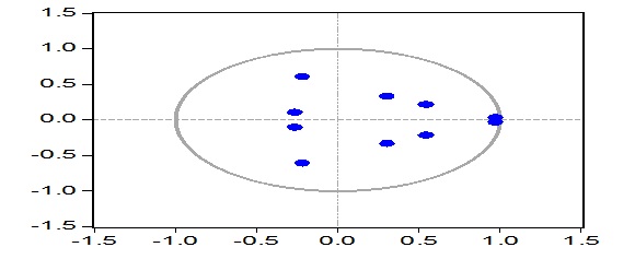
Fig.2: Inverse roots of the Autoregressive Polynomial. Johansen (1988)
cointegration test is applied to the VAR variables to test the
assumption that the five variables are bound by some long run phenomena,
though the variables might deviate from their short run relationship.
The trace and max tests for cointegration under the Johansen approach
show whether the null hypothesis of no cointegration vectors should be
rejected.
Ganger casuality tests were also applied to the estimated VAR
coefficients to determine the critical values of the block exogeneity
wald tests of the null hypothesis, that collectively the coefficients of
all the lags of a particular variable are simultaneously zero. The
rejection of the null hypothesis on the basis of the block exogeneity
tests suggests the variable(s) in the model which impact significantly
on the future values of each of the variables in the system. However,
causality tests only reveal the association among the variables and not
whether variance or change in value of a particular variable has a
positive or negative effect on other variables in the VAR system.
Therefore variance decomposition and impulse response function (IRF)
were estimated to examine the strength of such relationships within the
VAR system.
The estimated variance decomposition of RESDRENT, is the proportion
of the variance in RESDRENT that can be explained by its own shocks and
shocks to other variables. The forecast error variance (S.E) for an four
(4) period forecast horizon within the estimated variance decomposition
determines the proportion of RESDRENT for current and future periods (1,
2,3 and 4) which is accounted for by innovations to INFLATN, EXCHAG,
INTEREST and GDP. It is expected that the total percentage of the
forecast variance due to all innovations for each period sum up to 100.
Impulse response function (IRF) is further generated for the estimated
coefficients matrices in VAR model. The impulse response function traces
out the response of RESDRENT in the VAR system to shocks in the error
terms in equation
(1) to the extent that, if
in the RESDRENT
equation increases by one standard deviation, such change or shock will
change RESDRENT in the current and future periods.
5. RESULTS
The pairwise correlations in Table 4 show two important results.
First,residential property rents are strongly and positively correlated
with real GDP and exchange rates fluctuations in Nigeria. Secondly,
there are negative but weak correlations between residential property
rents and short–term interest rates as well as between residential
property rents and inflation rates. These results though a working
hypothesis, are later confirmed in the Variance decomposition within the
VAR framework later in this section.
Table 4. Pairwise Correlations of Variables at Zero Lag.
| Pairwise correlations at zero lag |
| |
GDP |
INFLATN |
EXCHAG |
INTEREST |
RESDRENT |
| GDP |
1 |
|
|
|
|
| INFLATN |
-0.31 |
1 |
|
|
|
| EXCHAG |
0.85 |
-0.38 |
1 |
|
|
| INTEREST |
-0.04 |
0.30 |
-0.02 |
1 |
|
| RESDRENT |
0.91 |
-0.34 |
0.91 |
-0.15 |
1 |
The Johansen cointegration test in Table 5shows the eigen value,
statistic, critical value and probability value at 5% level of
significance. By examining the trace test within the first two panels of
the table, null hypothesis of four cointegrating vectors at 5% level is
rejected as the trace statistics are greater than the critical values.
The max test shown in the other panel confirms this result.
On the basis of the granger causality test, it can be seen that with
the exception of inflation other macro economic variables forecast
RESDRENT. In this case all the lag coefficients of each of the
macroeconomic variables are statistically significant (p-values are less
than 5%) in the residential property rent equation, as indicated in the
last panel of table 6.
As a corollary, granger causality tests also show that while both the
short -term interest rates and exchange rates have significant effects
in the residential property rents, there is evidently ‘no reverse
significant’ of residential property rents on these two macroeconomic
variables ( their P Value are 0.2677 and 0.2838 respectively). These
results suggest that these two macroeconomic variables (short-term
interest rate and exchange rate) ‘granger cause’ residential property
rents and that these two macroeconomic variables have useful information
for predicting residential property rents over and above the past values
of other macroeconomic variables in the VAR model.
Table 5: Johansen Cointegration test for VAR Varaibles between 1984 -
2011
Unrestricted Cointegration Rank Test (Trace)
|
| Hypothesized |
|
Trace |
0.05 |
|
No. of CE(s)
|
Eigenvalue
|
Statistic |
Critical Value |
Prob.** |
| None * |
0.907094 |
134.6947 |
69.81889 |
0.0000 |
| At most 1 * |
0.706700 |
75.29040 |
47.85613 |
0.0000 |
| At most 2 * |
0.622274 |
44.62641 |
29.79707 |
0.0005 |
| At most 3 * |
0.527889 |
20.28673 |
15.49471 |
0.0088 |
At most 4
|
0.059109
|
1.523204
|
3.841466
|
0.2171
|
| Trace test indicates 4 cointegrating eqn(s) at
the 0.05 level |
| * denotes rejection of the hypothesis at the
0.05 level |
**MacKinnon-Haug-Michelis (1999) p-values
|
Unrestricted Cointegration Rank Test (Maximum
Eigenvalue)
|
| Hypothesized |
|
Max-Eigen |
0.05 |
|
| No. of CE(s) |
Eigenvalue
|
Statistic |
Critical Value |
Prob.** |
| None * |
0.907094 |
59.40431 |
33.87687 |
0.0000 |
| At most 1 * |
0.706700 |
30.66399 |
27.58434 |
0.0195 |
| At most 2 * |
0.622274 |
24.33968 |
21.13162 |
0.0171 |
| At most 3 * |
0.527889 |
18.76353 |
14.26460 |
0.0091 |
At most 4
|
0.059109
|
1.523204
|
3.841466
|
0.2171
|
| Max-eigenvalue test indicates 4 cointegrating
eqn(s) at the 0.05 level |
| * denotes rejection of the hypothesis at the
0.05 level |
| **MacKinnon-Haug-Michelis (1999) p-values |
Table 6: Granger Causality/ Block Exegeneity Wald Tests
Dependent variable: EXCHAG
|
| Excluded |
Chi-sq |
df |
Prob. |
| GDP |
2.372984 |
2 |
0.3053 |
| INFLATN |
1.762238 |
2 |
0.4143 |
| INTEREST |
1.794556 |
2 |
0.4077 |
RESDRENT
|
2.518923
|
2
|
0.2838
|
All
|
6.178470
|
8
|
0.6272
|
Dependent variable: GDP
|
| Excluded |
Chi-sq |
df |
Prob. |
| GDP |
0.733207 |
2 |
0.6931 |
| INFLATN |
0.440865 |
2 |
0.8022 |
| INTEREST |
2.984277 |
2 |
0.2249 |
RESDRENT
|
8.576370
|
2
|
0.0137
|
All
|
17.26949
|
8
|
0.0274
|
Dependent variable: INFLATN
|
| Excluded |
Chi-sq |
df |
Prob. |
| GDP |
0.365033 |
2 |
0.8332 |
| INFLATN |
0.603316 |
2 |
0.7396 |
| INTEREST |
0.674100 |
2 |
0.7139 |
RESDRENT
|
0.162122
|
2
|
0.9221 |
All
|
4.899009
|
8
|
0.7683
|
Dependent variable: INTEREST
|
| Excluded |
Chi-sq |
df |
Prob. |
| GDP |
0.835167 |
2 |
0.6586 |
| INFLATN |
2.085102 |
2 |
0.3526 |
| INTEREST |
9.443655 |
2 |
0.0089 |
RESDRENT
|
2.635744
|
2
|
0.2677
|
All
|
16.15057
|
8
|
0.0403
|
| Dependent variable: RESDRENT |
| Excluded |
Chi-sq |
df |
Prob. |
| GDP |
8.923314 |
2 |
0.0115 |
| INFLATN |
33.35944 |
2 |
0.0000 |
| INTEREST |
3.570942 |
2 |
0.1677 |
RESDRENT
|
10.34877 |
2
|
0.0057
|
All
|
46.27143
|
8
|
0.0000
|
Again, residential property rents and real GDP which are both
significant imply the existence of feedback relationship between real
GDP and residential property rents. The variance decomposition of
residential rents to shocks or innovations in macroeconomic variables in
Table 7 further confirms this result as it shows the contribution of
each macroeconomic shock to residential property rents.
Table 7: Variance Decompositions for Residential Property Rent
|
Period |
FORECAST ERROR VARIANCE (S.E) |
EXCHAG |
GDP |
INFLATN |
INTEREST |
RESDRENT |
| |
|
|
|
|
|
|
| 1 |
15.19901 |
0.000000 |
0.000000 |
0.000000 |
0.000000 |
100.0000 |
| 2 |
22.19551 |
6.951051 |
18.91081 |
0.023707 |
0.001505 |
74.11293 |
| 3 |
28.63879 |
9.285895 |
18.61029 |
0.087174 |
0.205616 |
71.81102 |
| 4 |
34.27057 |
14.10323 |
17.31054 |
0.485487 |
0.360693 |
67.74005 |
Cholesky ordering: RESDRENT INFLATN EXCHAG INTEREST GDP.
The forecast error variance (S.E) for four (4) years shows that real
GPD and Exchange ratetogether forecast 31.4% of the variance in
residential property rents. This result is consistent with those
reported in earlier studies byKeogh (1994) that GDP predicts the pattern
of rents and the findings of McCue and Kling, (1987); Kling and McCue,
(1994) that short- term interest rates contributes to the variation in
property returns performance. Finally, the Impulse Response Function
(IRF) as depicted in fig. 3shows that shocks to short-term interest
rates have a negative significant impact on residential property rents,
with the shocks getting a bit pronounced afterperiod two. Shocks or
innovations in inflation is negative but not significant and the shocks
die away instantly even at year zero. Increase in real GDP and exchange
rates have significant positive effects on residential rents. In this
case, rents appear to settle down quickly to a steady rising state after
period onedue to shocks of exchange rate and in the second period year
to shocks of real GDP.
6. CONCLUSIONS
Revisiting the interaction between the Nigerian property market and
the macroeconomy has further confirmed that the use of econometric
analysis rather adhoc methodologies purged with simple trend
interpolations is plausible. Since residential property rent is a
significant feature of most property market in the world, empirical
evidence based on this study from Nigeria implies that exogenous
influences of the economy (real GDP and Exchange rate) account for 31.4%
of the variation within the residential property market. At a
disaggregate level, real GDP accounts for a substantial proportion
(17.3%) of this variation in the residential property market, while
exchange rate account for the remaining 14.1% of these residential
property market variance. In addition the feedback mechanism between GDP
and residential property rents, means that these two variables are
determined contemporaneously and by implication depicts a somewhat
limited integration of the Nigerian residential property market with the
economy. The one to two period(s) response shocks of interest rate, real
GDP, and exchange rate show a relatively slow adjustment of the market
to the ever changing macroeconomic events in Nigeria. Such responses are
exogenous and make long run equilibrium within the residential property
market almost elusive. The existence of such analysis of this nature
will in the end aid useful property market analysis in a market fraught
with poor property market data.
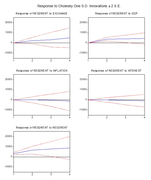
Fig.3. Responses of Residential Property Rent to Shocks in
MacroeconomicVariables.
REFERENCES
Barras, R. (1983). A simple theoretical model of the office
development cycle. Environment and Planning A, 15, pp.1381-1394.
Barras, R. (1994). Property and the economic cycle: building cycles
revisited. Journal of
Property Research, 11, pp. 183–197.
Barras, R., and Ferguson, D. (1985). A spectral analysis of building
cycles in Britain. Environment and Planning A, 17, pp.1369-1391.
Barras, R., and Ferguson, D. (1987a). Dynamic modelling of the building
cycle 1: theoretical framework. Environment and Planning A, 19, pp.
353–367
Barras, R., and Ferguson, D. (1987b). Dynamic modelling of the building
cycle 2: empirical
results. Environment and Planning A, 19, pp. 493–520.
Brooks, C. (2008). Introductory econometrics for finance. 2nd ed. New
York: Cambridge University Press.
Brooks, C., and Tsolacos, S. (1999). The impact of economic and
financial factors on UK property performance. Journal of Property
Research, 16(2), pp. 139–152.
Chan, K.C., Hendershott, P.H. & Sanders, A.B. (1990). Risk and return on
real estate:
evidence from equity REITs. American Real Estate and Urban Economics
Association Journal, 18, pp. 431-452.
Dehesh, A., and Pugh, C. (1995). Property cycle in a global economy.
Urban studies, 37(13)
pp.2581-2602.
Diebold, F.X. (2001). Elements of forecasting. 2nd ed. South Western
Publishing.
DiPasquale, D., and Wheaton, W.C. (1996). Urban economics and real
estate markets. New-
Jersey: Prentice-Hall, Inc. Englewood Cliffs.
Geltner, D. M., Miller, N. G., Clayton, J. & Eichholtz, P. (2007),
Commercial real estate
analysis and investments, 2nd ed.Thomson South-Western.
Giussani, B., Hsai, M. & Tsolacos, S. (1992). A comparative analysis of
the major determinants of office rental values in Europe.Journal of
Property Valuation and Investment, 11(2), pp.157–173.
Gujarati, D. N. (2003). Basic econometrics. 4th ed. New York:
McGraw-Hill
Hartzell, D., Hekman, J.S. & Miles, M.E. (1987). Real estate returns and
inflation. American Real Estate and Urban Economics Association Journal,
15(1), pp. 617-637.
Hekman, J.S. (1985). Rental price adjustment and investment in the
office market. American Real Estate and Urban Economics Association
Journal, 13(1), pp. 32-47.
Hetherington, J.T. (1988). Forecasting of rents. In: A. MacLeary and N.
Nathakumaran,
eds.Property investment theory, UK: Spon.
Hoag, J.W. (1980). Towards indices of real estate value and return.
Journal of Finance, 35(2), pp 569-580.
Johansen, S. (1988). Statistical analysis of cointegrating vectors.
Journal of Economic Dynamics and Control, 12, pp. 231-254
Joshi, H. (2006). Identifying asset price bubbles in the housing market
in India- preliminary evidence. Reserve Bank of India Occasional Papers
27, pp. 73–88.
Keogh,G. (1994). Use and investment markets in British real estate.
Journal of Property Valuation and Investment, 12(4), pp 58-72.
Kling, J.L., and McCue, T.E. (1987). Office building investment and the
macroeconomy: empirical evidence, 1973-1985. American Real Estate and
Urban Economics Association Journal, 15(3), pp.234-255.
Kling, J.L., and McCue, T.E. (1991). Stylized facts about industrial
property construction. Journal of Real Estate Research, 6(3),
pp.293-304.
Koop, G. (2000). Analysis of economic data. New York: John Wiley and
Sons.
Ling, D., and Naranjo, A. (1997). Economic risk factors and commercial
real estate returns, Journal of Real Estate Finance and Economics,
14(3), pp. 283-307.
Ling, D., and Naranjo, A. (2003). The dynamics of REIT capital flows and
returns, Real Estate Economics, 31, pp. 405–434.
Lizieri, C., and Satchell, S. (1997a) Interactions between property and
equity markets: an investigation of linkages in the UK 1972-1992.
Journal of Real Estate Finance and Economics, 15(1), pp.11-26.
Lizieri, C., and Satchell, S. (1997b) Property company performance and
real interest rates: a regime switching approach. Journal of Property
Research, 15, pp. 85-97.
Lutkepoh, H. (1991)Introduction to Multiple Time Series Analysis, New
York: Springer-Verlag.
McCue, T.E., and Kling, J.L. (1994) Real estate returns and the
macroeconomy: some
empirical evidence from real estate investment trust data, 1972-1991,
Journal of Real
Estate Research 9(3), pp. 277-287.
Ojetunde, I., Popoola, N.I., and Kemiki, O.A. (2011). On the interaction
between the Nigerian residential property market and the macroecconomy.
Journal of Geography,Environment and Planning, 7(2), University of
Adoekiti, Nigeria.
Stiglitz, J. (1994). The role of the state in financial markets. In: M.
Bruno and R. Pleskovic, eds. Proceedings of the World Bank Annual
Conference on Development Economics 1993, pp. 19–56. Washington, DC:
World Bank.
Viezer, T.W.(1999). Econometric integration of real estate’s space and
capital markets. Journal of Real Estate Research, 18(3).
Vishwakarma, V.K., and French, J.J. (2010). Dynamic linkages among
macroeconomic factors and returns on the Indian real estate sector.
International Research Journal of Finance and Economics, 43.
CONTACT
Ismail Ojetunde
Federal University of Technology, Minna. Nigeria
P. M. B. 65 Minna, Niger State of Nigeria
Minna
NIGERIA
Tel: + 2347033780000
Email:
i.ojetunde@futminna.edu.ng,
ismajet2003@yahoo.com
 |