Article of the
Month - March 2021
|
Macrotidal Beach Monitoring (Belgium) using
Hypertemporal Terrestrial Lidar
Greet Deruyter, Lars De Sloover, Jeffrey Verbeurgt, Alain De Wulf,
Belgium And Sander Vos, The Netherlands
 |
 |
 |
 |
 |
| Greet Deruyte |
Lars De Sloover |
Jeffrey Verbeurgt |
Alain De Wulf |
Sander Vos |
This article in .pdf-format (13pages)
This article was included in the proceedings of FIG Working Week
2020. Knowledge on natural sand dynamics is essential and the
authors present first results achieved with currently used
methodology. Next, they analyze the results from a 10-day
measurement campaign and highlight the tide-dominated beach
morphology.
SUMMARY
In order to protect the Belgian coast, knowledge
on natural sand dynamics is essential. Monitoring sand dynamics is
commonly done through sediment budget analysis, which relies on
determining the volumes of sediment added or removed from the coastal
system. These volumetrics require precise and accurate 3D data of the
terrain on different time stamps. Earlier research states the potential
of permanent long-range terrestrial laser scanning for continuous
monitoring of coastal dynamics. For this paper, this methodology was
implemented at an ultradissipative macrotidal North Sea beach in
Mariakerke (Ostend, Belgium). A Riegl VZ-2000 LiDAR, mounted on a 42 m
high building, scanned the intertidal and dry beach in a test zone of
ca. 200 m wide on an hourly basis over a time period of one year. It
appeared that the laser scanner could not be assumed to have a fixed
zenith for each hourly scan. The scanner compensator measured a variable
deviation of the Z-axis of more than 3.00 mrad. This resulted in a
deviation of ca. 900 mm near the low water line. A robust calibration
procedure was developed to correct the deviations of the Z-axis. In this
paper, we start by presenting the first results achieved with the
current methodology. Next, we analyze the results from a 10-day
measurement campaign and highlight the tide-dominated beach morphology.
1. INTRODUCTION
Terrestrial LiDAR (Light Detection And Ranging) technology makes it
possible to collect high resolution, accurate and instantaneous
topographic data of large areas. In the last decade, terrestrial laser
scanning (TLS) has been more and more used to study aeolian and coastal
geomorphology (Almeida et al., 2013; Huising & Gomes Pereira, 1998;
Montreuil, Bullard, & Chandler, 2013; Pye & Blott, 2016).
Lindenbergh et al. (Lindenbergh, Soudarissanane, de Vries, Gorte, &
de Schipper, 2011) presented short-range static terrestrial laser
scanning on a beach to identify morphodynamic changes at the
sub-centimeter level. More recently, Anders et al. and Vos et al.
(Anders et al., 2019; Vos, Lindenbergh, & De Vries, 2017) described the
use of permanent TLS (range < 300 m) for continuous (hypertemporal)
monitoring of coastal change. Their study set-up determined a precision
in terms of a standard deviation of 1.5 cm between two-consecutive
scans.
The study area and system configuration of the laser scanner are
elaborated in the second section. The third section describes the
different alignment and calibration methods used. Section 4 assesses the
results of the calibration procedures as well as some findings from a
10-day case study.
2. STUDY AREA & SYSTEM CONFIGURATION
In this study, the methodology developed by Vos et al. (Vos et
al., 2017) was implemented at the North Sea beach of Mariakerke (Ostend,
Belgium) (figure 1 & figure 2 – left panel) using a Riegl® VZ-2000
terrestrial laser scanner. A seawall (figure 1) and a groin field (200 m
between each groin) with regularly carried out beach and underwater
nourishments characterize this beach. It is gently sloping (1 – 2 %) and
ultra-dissipative (Deronde, Houthuys, Henriet, & Van Lancker, 2008),
consisting of medium and coarse sand with an average grain size of 310
µm. The Belgian coast is situated in a macro-tidal regime ranging from
3.5 m at neap tide to 5 m at spring tide. The area of interest is
bordered by the two groins and the seawall. Over the past few years,
this beach has been the subject of frequent mobile and static
terrestrial LiDAR surveys (De Wulf, De Maeyer, Incoul, Nuttens, & Stal,
2014; Stal et al., 2014).
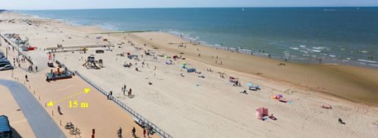
Figure 1. Mariakerke Beach and its typical
seawall at mid-tide.
In our field set-up, the vertical axis of the laser scanner appears
to have a certain variability between hourly scans of more than 3.00
mrad, resulting in a shift of more than 0.9 meter at the low water line.
The aim of this study was to develop a robust and automated alignment
procedure to adjust both the hourly and fixed deviations of the
scanner’s zenith. The final objective is to examine which combination of
calibration parameters yields the best results.
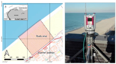
Figure 2. Map of the study area (left), Riegl®
VZ-2000 TLS overlooking the beach (right)
A time-of-flight pulse-based laser scanner, mounted on a 42 m high
building near the study area (figure 2, right panel), scanned the
intertidal and dry beach. The scanner was installed on a stable frame
and protected by weather-proof housing. The exact scanner location was
determined through Real-Time Kinematic Global Navigation Satellite
System (RTK-GNSS) positioning. Data acquisition took place on an hourly
base from 8 November 2017 to 6 December 2018.
3. METHODOLOGY
The deviation of the vertical axis of the scanner required the
development of a robust and automated calibration procedure to correct
both the hourly and fixed deviations of the scanner’s Z-axis. The
variables of the problem are the inclination of the Z-axis in two
different preferably independent directions. For easy intuitive
interpretation, the orthogonal directions of the seawall (X-axis) and
the groin (Y-axis) were selected.
A static scan produces a dense point cloud, containing around four
million points, with approximately one million situated on the seawall
and groin, one million points on the dry beach and one million in the
intertidal zone. Environmental constraints (e.g. high humidity of the
surface, rain, fog, snow or high tide) yield smaller point sets on the
beach.
The actual calibration procedure is done by making a 2.5D model of
each static scan and registering it to a ‘truth’ set of reference
points. The robustness of the alignment implies that the calibration
procedure must approximate the following ideal situation:
- Independence of the model used and the parameters applied to
build the model (3.1.)
- Independence of the truth set of reference points (3.2.);
- Independence of the outlier elimination strategy (3.3.).
3.1. Model Selection
For the scan-based model, two main approaches were used:
- Triangulated Irregular Network (TIN) or mesh modelling: Delaunay
2.5D triangulation within the convex hull. If an unlimited maximum
length for the triangle edges is given, then all triangles output by
the triangulation will be kept. Specifying a maximum edge length as
parameter allows to remove the biggest triangles that are not
necessarily meaningful.
- Grid modelling: the height of each grid cell is computed by
averaging the elevation of all points included in this cell. If a
given cell contains no points, this cell will be considered as
‘empty’. The cell size is the variable applied parameter.
3.2. Reference Data Selection
For the choice of truth, three sets of reference points were
available:
- ALS: an airborne LiDAR scan (ALS) acquired on the same day and
timestamp as the static scan of around one million points with an
average point density of around 2 points/m², resulting in a
reference set of 3777 points.
- RTK-GNSS: a set of 800 RTK-GNSS reference points on the seawall
and the groin.
- SfM-MVS: image-based modelling (Structure from Motion-Multi-View
Stereo), acquired via UAV on the same day and timestamp as the
static scan and the LiDAR flight resulted in a reference set of
around 3684 points.
Figure 4 shows the workflow applied. Either a
TIN model or a gridded model of the static scan was made. In case of the
TIN-approach, the difference between the scan model and the truth set is
the height difference between individual points of the reference set and
the corresponding triangle of the TIN-model of the scan. In the
grid-approach, grids of both the scan and the reference set were made.
However, the static scan yields different point densities at the end of
the groin compared to the end of the seawall. For this reason, the
interval distance for the rasterizing was chosen differently in the
seawall zone compared to the groin zone to obtain a balanced calibration
set in the x- and y-direction. Next, using a Monte Carlo simulation with
multiple rotational values, the difference between the scan model and
the reference set was minimized. From an angle of -5 mrad till + 5 mrad,
1001 x-axis rotational values are combined with 1001 y-axis rotational
values in steps of 0.01 mrad.
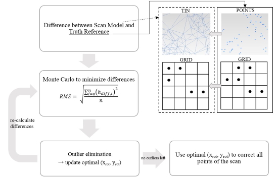
Figure 4. Workflow of the calibration algorithm.
3.3. Outlier Elimination Strategy
Each static scan is expected to contain
outliers. The outliers originate mainly from ghosting (e.g. people and
obstacles on the seawall and groin that are scanned). These outliers
yield elevation values that are significantly higher than the true
surface. A severe outlier test is needed, but eliminating too many
values gives a too optimistic value in terms of calibration quality. A
point i of the reference set is an outlier if
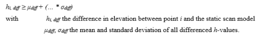
Finally, a sigma rule of thumb is applied, considering a width of 2,
2.5 and 3 standard deviations around the mean. After each elimination of
outliers, an optimal x- and y-rotation are computed, yielding slightly
different values as the reference set was modified in the previous step
and subsequently a new outlier test is performed. This iterative process
continues till no more outliers are detected. If no more outliers can be
detected, all the points of the static scan are corrected with the
optimal x- and y-rotation.
4. RESULTS
Table 1 gives an overview of the calibration quality statistics per
model of the static scan and model parameter applied for a first series
of calibration runs with a selection of the 50 most accurate points in
the truth. The mean of algebraic differences (MEAN), the mean of
absolute differences and the RMS are calculated for each model parameter
individually. Per static scan model and per parameter, the applied
rotation around the x- and y-axis are given.
Table 1. Static scan models and parameters
applied –mean of algebraic differences (MEAN), mean of absolute
distances, RMS, and x- & y-axis rotation for a first series of
calibration runs.
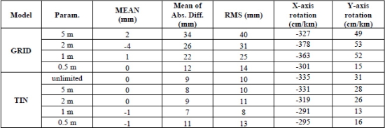
The TIN models (5 m, 2 m, 1 m and unlimited edge
size) perform best in all categories. From here on, these models were
used in the quest for the best reference set and the optimal outlier
elimination strategy. For each reference set, the three-sigma (2, 2.5
and 3 standard deviations) outlier elimination tests were done plus a
test without outlier elimination. In order to make a clear and easy
comparison, one weighted (considering all TIN parameters) RMS (figure 5,
panel A) were calculated for all outlier elimination strategies per
reference set.
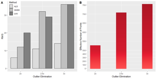
Figure 5. Visualization of RMS as a function of
n·sigma per reference set (A) and number of effective points used as a
function of n·sigma for the ALS reference set (B).
Figure 5 (B) shows the effective number of
points used per outlier elimination strategy for the ALS reference set.
An outlier elimination strategy of 2.5σ gives a good overall result with
not too many points eliminated and sufficient effective points
remaining.
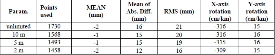
Table 2 gives an overview of the MEAN, Mean of
Absolute Differences, RMS and x- & y-axis rotation for different edge
limit values of the TIN model, calibrated on the ALS truth with 2.5σ
outlier removal.
Table 2. Statistics of the calibration procedure
for different TIN sizes
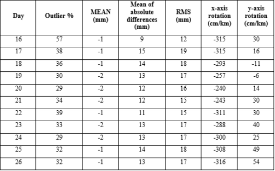
As a case study, calibration results of a 10-day
measurement campaign from 16 April 2018 till 26 April 2018 were
analyzed. Different parameters were taken into consideration, including
outlier percentage (effective number of points used divided by the
initial amount of points in the point cloud), mean of algebraic
differences, mean of absolute differences, RMS and x- and y-axis
rotation. The results of this 10-day study are presented in Table 3.
Table 2. Statistics of the calibration procedure
for 10 consecutive days.
During this campaign, meteorological conditions
(both aeolian and hydrodynamic forcing) were observed at the nearby
Ostend Meteo Park and the Raversijde Waverider Buoy. Wind and wave data
of the 10-day period are presented in figure 6 and 7 below.
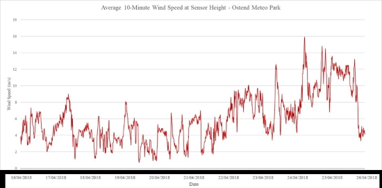
Figure 6. Results from wind speed measurements
(temporal resolution = 10 minutes) at the Ostend Meteo Park.
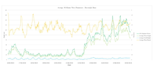
Figure 7. Results from wave measurements
(temporal resolution = 30 minutes) at the Raversijde Buoy.
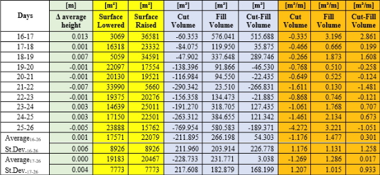
Additionally, volume changes within a fixed study area were
determined between the first (16 April 2018) and last day (26 April
2018) of the campaign, using a so called planimetric method, based on
the TIN-interpolated scan model. Table 3 below shows the change in daily
average height of the beach surface within the study area, as well as
the daily changes in volume.
Table 3. Changes in volume and average height of
the beach surface in-between consecutive days.
5. DISCUSSION
The higher the resolution of the grid model, the more accurate the
computation of the difference in heights between the static scan model
and the reference points. The smaller the cell / edge limit value, the
more holes in the model, the less reference points can be interpolated
in the model, reducing the quantity and therefore the validity of the
difference point set. Overall, the TIN model yields the most means of
algebraic differences close to zero, this is thus a good measure of
accuracy. The TIN-model (10 m, 5 m, 2 m and unlimited edge size) has the
smallest mean of algebraic differences and the smallest RMS and are
therefore the most precise (repeatable) models with the smallest random
error.
Hence, for further processing, only the TIN-model with 10 m, 5 m, 2 m
and unlimited edge size were considered. On one hand, it can be easily
concluded that the ALS truth yields the best overall RMS for all TIN
models together (figure 5-A). It shows on the other hand that the GNSS
reference set with 2σ elimination returns a similar RMS. Figure 5-B
however shows that the outlier removal percentage for 2σ is way higher
than 2.5σ with both GNSS and ALS. Moreover, less points available in the
reference set, reduces the quantity and therefore validity of the
calibration.
When looking closer at the results (table 2) for different edge limit
values of the TIN with 2.5σ outlier elimination and ALS truth, several
remarks can be made. The applied rotation (in both directions) is more
or less the same for all edge limit values. The TINs with smaller edge
limit values produce a lower RMS and mean of absolute differences but
yield a smaller reference set available for the model interpolation. At
the same time, the TINs with bigger edge limit values have less points
eliminated, but come with a higher RMS and mean of absolute differences.
A TIN with 5 m edge limit value seems to be the middle ground with an
RMS of 19 mm, and an accuracy of 15 mm.
Interpretation of the aeolian and hydrodynamic forcing shows calm
conditions during the first days (16 till 21 April) with wave heights
below 80 centimeters and wind speeds only incidentally exceeding the 7
m/s threshold for aeolian transport. Swell and wave period conditions
remain constant throughout the entire 10-day period. From 22 April till
26 April, wind speeds exceeded the 7 m/s on a few occasions and average
wave heights were as high as 140 centimeters (with outliers reaching up
to 180 centimeters).
An analysis of Table 2 (reporting the day-to-day calibration results)
leads to a number of conclusions. First of all, the x-axis deflection
varies between -316 and -240 cm/km with a maximal daily variation of 68
cm/km. Y-axis deflections vary between -11 and 54 cm/km with a maximal
daily variation of 27 cm/km. A trendline nor a correlation with aeolian
forcing could, at first sight, not be detected.
When looking at the RMS values of the differences between the
reference aerial LiDAR point cloud and the calibrated static scan TIN
model, variations between 12 and 19 mm occur. The lowest RMS (12 mm) was
observed on the first day. This can be explained by a lower number of
reference points that could be interpolated in the TIN model. 16 April
was a rainy day, leading to a sparser coverage scan points on the dike
and groin.
Finally, it appears that the daily means of absolute deviations are
not symmetrically distributed around zero. The static scan model lies
systematically above the height of the reference data sets, which is to
be expected as obstacles (e.g. ghosting) are all above the surface of
the dike and groin reference points.
The volume changes in our area of interest during the campaign are
small. Between the first (16 April) and last day (26 April), there is an
increase in average height of the beach of 14 mm. The maximum difference
between successive days is 13 mm between 16 April and 17 April,
corresponding to a net volume change of + 515.688 m³ or 2.861 m³/m.
Between the other successive days, the maximum absolute difference of
the average height is only 7 mm with a standard deviation of differences
of 4 mm. When ignoring the first day; the net volume change between
successive days varies between -1.481 m³/m and + 1.608 m³/m, yielding an
average cut-fill volume of just (0.017 ± 0.933) m³/m.
Despite the calm environmental forcings during the first days of the
campaign, a significant change of the beach topography occurs. The last
days of the campaign are characterized by higher waves and stronger
winds. However, no significant changes in beach topography take place.
When looking at the tides; spring tide occurred at 16 April. It
appears the highest changes in intertidal beach topography take place
during more extreme tidal conditions. When the tidal conditions are
‘calm’, beach topography remains the same, despite higher waves and
stronger winds.
6. CONCLUSION
Recently, terrestrial LiDAR and permanent TLS have been more and more
used to monitor coastal morphodynamics. However, these sorts of
experiments come with the demand for an accurate calibration. In this
study, a robust and automated alignment procedure was developed to
correct deviations of the scanner’s zenith. Besides, each static scan is
expected to contain altimetric outliers, originating from ghosting.
Different 2.5D models of one scan were registered to different sets of
reference points. Ultimately, several iterative outlier elimination
procedures were tested. Modelling the static scan into a TIN with
triangle edge sizes no longer than 5 metres yielded the best results for
a calibration on the ALS reference data set. A 2.5σ outlier elimination
gave the best accuracies. As a case study, a 10-day measurement campaign
was set up. During this campaign, both spring and neap tide took place.
Calm wave conditions without wind occured as well as stronger winds and
higher waves. Finally, it can be assumed that during the period of 17 –
26 April no significant volume changes took place on the beach and that
any (small) variation in beach topography is due to measurement errors
of the LiDAR. Future research will focus on the processing of
multi-temporal scan series with a view to the detection of coastal
morphological features.
REFERENCES
- ADDIN Mendeley Bibliography CSL_BIBLIOGRAPHY Almeida, L. P.,
Masselink, G., Russell, P., Davidson, M., Poate, T., McCall, R., …
Turner, I. (2013). Observations of the swash zone on a gravel beach
during a storm using a laser-scanner (Lidar). Journal of Coastal
Research, 65, 636–641. https://doi.org/10.2112/si65-108.1
- Anders, K., Lindenbergh, R. C., Vos, S. E., Mara, H., De Vries,
S., & Höfle, B. (2019). High-Frequency 3D Geomorphic Observation
Using Hourly Terrestrial Laser Scanning Data of A Sandy Beach. ISPRS
Annals of the Photogrammetry, Remote Sensing and Spatial Information
Sciences, 4(2/W5), 317–324.
https://doi.org/10.5194/isprs-annals-IV-2-W5-317-2019
- Brand, E., De Sloover, L., De Wulf, A., Montreuil, A.-L., Vos,
S., Chen, M., … Chen, M. (2019). Cross-Shore Suspended Sediment
Transport in Relation to Topographic Changes in the Intertidal Zone
of a Macro-Tidal Beach (Mariakerke, Belgium). Journal of Marine
Science and Engineering, 7(6), 172.
https://doi.org/10.3390/jmse7060172
- De Wulf, A., De Maeyer, P., Incoul, A., Nuttens, T., & Stal, C.
(2014). Feasibility study of the use of bathymetric surface
modelling techniques for intertidal zones of beaches. FIG Working
Week, (June 2014), 8.
- Deronde, B., Houthuys, R., Henriet, J. P., & Van Lancker, V.
(2008). Monitoring of the sediment dynamics along a sandy shoreline
by means of airborne hyperspectral remote sensing and LIDAR: A case
study in Belgium. Earth Surface Processes and Landforms, 33(2),
280–294. https://doi.org/10.1002/esp.1545
- Huising, E. J., & Gomes Pereira, L. M. (1998). Errors and
accuracy estimates of laser data acquired by various laser scanning
systems for topographic applications. ISPRS Journal of
Photogrammetry and Remote Sensing, 53(5), 245–261.
https://doi.org/10.1016/S0924-2716(98)00013-6
- Lindenbergh, R. C., Soudarissanane, S. S., de Vries, S., Gorte,
B. G. H., & de Schipper, M. A. (2011). Aeolian Beach sand transport
monitored by terrestrial laser scanning. Photogrammetric Record,
26(136), 384–399. https://doi.org/10.1111/j.1477-9730.2011.00659.x
- Montreuil, A.-L., Bullard, J., & Chandler, J. (2013). Detecting
Seasonal Variations in Embryo Dune Morphology Using a Terrestrial
Laser Scanner. Journal of Coastal Research, 165(65), 1313–1318.
https://doi.org/10.2112/si65-222.1
- Pye, K., & Blott, S. J. (2016). Assessment of beach and dune
erosion and accretion using LiDAR: Impact of the stormy 2013–14
winter and longer term trends on the Sefton Coast, UK.
Geomorphology, 266, 146–167.
https://doi.org/10.1016/J.GEOMORPH.2016.05.011
- Stal, C., Incoul, A., De Maeyer, P., Deruyter, G., Nuttens, T.,
& De Wulf, A. (2014). Mobile mapping and the use of backscatter data
for the modelling of intertidal zones of beaches. International
Multidisciplinary Scientific GeoConference Surveying Geology and
Mining Ecology Management, SGEM, 3(2), 223–230.
- Vos, S., Lindenbergh, R., & De Vries, S. (2017). CoastScan:
Continuous Monitoring of Coastal Change Using Terrestrial Laser
Scanning. Coastal Dynamics, (233). Retrieved from www.ahn.nl
BIOGRAPHICAL NOTES
CONTACTS
MSc Lars De Sloover
Ghent University, Department of Geography
Krijgslaan 281 (S8 Building)
9000-GhentBELGIUM
Web site:
www.geografie.ugent.be/members/802002047140
Prof. dr. ing. Greet Deruyter
Ghent University, Department of Civil Engineering
Msc Lars De Sloover
Ghent University, Department of Geography
Msc Jeffrey Verbeurgt
Ghent University, Department of Geography
Prof. dr. ir. Alain De Wulf
Ghent University, Department of Geography
Dr. ir. Sander Vos
Delft Technical University, Department of Hydraulic Engineering, the
Netherlands
Email: S.E.Vos@tudelft.nl


