FIG PUBLICATION NO. 25
models
and terminology for the analysis of geodetic monitoring observations
Official Report of the Ad-Hoc Committee of FIG Working
Group 6.1
Prof. Walter M. Welsch, Institute of Geodesy, Bundeswehr
University Munich, Germany
Prof. Otto Heunecke, Geodetic Institute, University of
Hannover, Germany
CONTENTS
PREFACE
ABSTRACT
1. HISTORY AND INTRODUCTION
2. CONCERN OF
DEFORMATION MEASUREMENTS
3. CONVENTIONAL
DEFORMATION ANALYSIS
3.1 Congruence Models
3.2 Kinematic Models
4. DYNAMIC SYSTEMS AND ADVANCED DEFORMATION
ANALYSIS - SYSTEMATIZATION OF DEFORMATION MODELS
5. SYSTEM IDENTIFICATION BY
PARAMETRIC AND NON-PARAMETRIC MODELS
5.1 Parametric models
5.2 Non-parametric models
6. SOME EXAMPLES OF APPLICATION
6.1 General Procedure
6.2 Example Using a Parametric Model
6.3 Non-parametric Input-Output Model of a Turbine Foundation
6.4 Integrated Parametric Analysis of Ground Subsidence
7. POTENTIALITY OF DYNAMIC MODELS
8. CONCLUSION
REFERENCES
Orders of the printed copies
It is my great pleasure, as the chairman of FIG Working Group 6.1
(Deformation Measurements), to introduce to the members of FIG this final
report of the ad hoc Committee on Terminology and Classification of
Deformation Models. I would like to thank Dr. Walter Welsch and Dr.
Otto Heunecke for undertaking the difficult task of summarizing the
results of 8 years of research and discussions (sometimes heated) on the
subject within the activity of WG 6.1. The need for the special study of the
classification and terminology used in deformation modeling was recognized
at the 6th International Symposium organized by the FIG WG 6.1 (formerly
known as WG6C) in Hanover, Germany, in 1992. The need arose as a result of
the growing interest in the interdisciplinary approach to physical
interpretation and modeling of the relationship between causative factors
(loads) and deformation. Though basics of the load-deformation analysis are
well known in applied physics and mechanics of deformable bodies, geodetic
engineers have entered the discipline only recently. At the symposium in
Hanover, some authors became confused with the use of the terms such as
dynamic or kinematic models of deformation, deterministic vs. statistical,
or parametric vs. non-parametric modeling, etc. Though this final report may
not satisfy all specialists in deformation modeling, who may be coming from
various fields of science and engineering, it gives geodetic engineers a
solid basis for a unification of terms used in deformation modeling.
Certainly, there will be still more discussion on the subject but the
background gained from this report will help geodetic engineers to better
understand the finesses of the modeling processes.
This report represents one of the latest involvements of Working Group
6.1.The group has always been one of the most vital groups of FIG Commission
6 and one of the most active international groups dealing with the problems
of monitoring and analysis of deformation surveys in engineering and
geoscience projects. Although the accuracy and sensitivity criteria for
determining deformations may considerably differ between various
applications, the basic principles of the design of monitoring schemes and
their analysis remain the same.
Due to the constantly growing technological progress in all fields of
engineering and, connected with it, the increasing demand for higher
accuracy, efficiency, and sophistication of the deformation measurements,
geodetic engineers have to continuously search for new monitoring techniques
and have to refine their methods of deformation analysis. Working Group 6.1
has played a very important role in providing a forum for the exchange of
information in the new developments by organising ad hoc study groups,
technical sessions during the FIG Congresses and, more important, by
organising specialised international symposia on deformation surveys. These
have occurred in 1975 in Krakow, Poland, in 1978 in Bonn, Germany, in 1982
in Budapest, Hungary, in 1985 in Katowice, Poland, in 1988 in Fredericton,
Canada, in 1992 in Hanover, Germany, in 1993 in Banff, Canada, in 1996 in
Hong Kong, in 1999 in Olsztyn, Poland, and (the 10th symposium) in Orange,
California, in 2001. The published proceedings of those symposia provide an
enormous wealth of information on the development of new techniques and new
methods in monitoring and analysis of deformations. The next symposium is
planned to be held in Greece in 2003.
Professor Adam Chrzanowski
Chairman, FIG Working Group 6.1 - Deformation Measurements
MODELS
AND TERMINOLOGY FOR THE ANALYSIS
OF GEODETIC MONITORING OBSERVATIONS
Official Report of the Ad-Hoc Committee of FIG Working
Group 6.1
Walter M. Welsch
Institute of Geodesy
Bundeswehr University Munich
D-85577 Neubiberg
Germany
Otto Heunecke
Geodetic Institute
University of Hannover
D-30167 Hannover
Germany
The paper in hand is the result of the studies of the Ad-Hoc Committee
'Classification of Deformation Models and Terminology' of Working Group 6.1
'Deformation Measurements', FIG Commission 6. The Ad-Hoc Committee was set
to work due to a recommendation of the chair-man of FIG-Working Group 6.1 on
the occasion of the 6th International FIG-Symposium on De-formation
Measurements in Hannover in 1992. Earlier reports were given on the 7th
International FIG-Symposium on Deformation Measurements in Banff, Canada in
1993, on the Perelmuter Workshop on Dynamic Deformation Models in Haifa,
Israel in 1994, and in 1996 at the 8th International FIG-Symposium on
Deformation Measurements in Hong Kong. A summary of the studies was
presented at the 9th FIG-Symposium on Deformation Measurements in Olsztyn,
Poland in 1999. The closing session of this symposium was devoted to a
comprehensive discussion on the topic. It was concluded by the chairman of
Working Group 6.1 summarizing the activities concerning the methods and
models of deformation analysis during the past two decades. The paper here
as submitted to the 10th FIG International Symposium on Deformation
Measurements in Orange, California in 2001 is the official final report of
the Ad-Hoc Committee and includes the proposals discussed in Olsztyn.
A summary of the studies can be described as follows: The deformation of
an object is the result of a process. The today's techniques offer the
possibilities to measure and analyze such a process in all details. This is
in accordance with the current trends in engineering surveying which intend
to determine not only the geometrical changes of an object in a
phenomenological manner but rather the dynamics of the process, i.e. the
investigations aim at incorporating the causative forces and the physical
properties of the body. In its entirety, the body, the causative forces and
the resulting deformations are considered a dynamic system. Consequently,
the most general and comprehensive models are dynamic models, from which -
by simplification - static, kinematic and congruence models are derived. The
simplified models offer the possibility of meeting many practical aspects of
deformation analysis which do not necessarily require the complete
investigation of the process in all details.
As a result it can be stated that in our days 'geodetic deformation
analysis' means 'geodetic analysis of dynamic processes'. The tools to do
so, are made available by disciplines like e.g. the sciences of civil
engineering, mechanics, filter and control engineering, signal analysis, and
system theory. Especially system theory provides an established terminology
and classification of models for an up-to-date deformation analysis in the
above sense and in accordance with the latest trends of engineering
surveying. Deformation analysis should be considered an interdisciplinary
concern to the benefit of all sciences involved.
In the late 1970s and early 1980s, Working Group 6.1 of FIG concentrated
their efforts on the development of new monitoring techniques and on the
geometrical analysis of frequently ob-served geodetic deformation networks,
continuous measuring techniques were just at the beginning. This state is
reflected e.g. in the content of the papers presented at the 1st
FIG-Symposium on Deformation Measurements in Krakow (1975). At that time,
the main problem of the deformation analysis was the identification of
unstable reference points in geodetic monitoring networks. Several
approaches were proposed by different authors. As a result, an Ad-Hoc
Committee on Deformation Analysis was established at the 2nd Symposium in
Bonn (1978) with the task of comparing different approaches and developing a
unified theory for the geometrical analysis of deformation surveys. Several
research centers joined the work of the committee, with the most active
centers being from universities of Karlsruhe, Hannover, Stuttgart, and
Munich in Germany, universities of New Brunswick in Canada, and Delft in the
Netherlands. The work of the Committee was summarized at the XVI.
FIG-Congress in Montreux (Chrzanowski et al. 1981), at the 3rd Symposium on
Deformation Measurements in Budapest (Heck et al. 1982), at the XVII.
FIG-Congress in Sofia (Chrzanowski and Secord 1983), and at the XVIII.
FIG-Congress in Toronto (Chrzanowski and Chen 1986).
Parallel to the work of the Ad-Hoc Committee on Deformation Analysis,
several researchers especially at the universities in Stuttgart
(Felgendreher 1981, 1982), Hannover (Boljen 1983, 1984), in Fredericton
(Chrzanowski et al. 1982; Chen 1983; Chrzanowski et al. 1986; Chen and
Chrzanowski 1986), in Calgary (Teskey 1986, 1988), and in Munich (Ellmer
1987; Kersting 1992) initiated work on expanding the deformation analysis
into the physical interpretation and modeling of the relationship between
causative factors (loads) and the resulting deformations. Some authors began
already to take advantage of the increasing importance of automated
measuring techniques (e.g. Pelzer 1977a, 1977b, 1978). The work of these
researchers was fundamental for the development of geodetic deformation
analysis to a deeper and wider understanding of deformation phenomena which
are basically the result of dynamic processes. It was understood that
deformation analysis has basically to be seen from an interdisciplinary
point of view. Consequently the field of geodetic deformation analysis
expanded, e.g. into civil engineering and geotechnical applications.
The more geodesists and engineering surveyors went into the analysis of
dynamic processes, the more confusing were the technical terms they were
applying to their studies. The terminology which could have been used was
well established in physics and mechanics and in other sciences a long time
before geodetic engineers became involved in the physical interpretation of
deformation. In 1992, at the 6th FIG-Symposium in Hannover, some papers made
the confusion obvious: e.g. the purely geometrical analysis of deformation
measurements was called 'static' by some authors, or the time dependent
geometrical analysis was named 'dynamic', particularly when dealing with
cyclically changeable deformations etc. The main confusion arose from the
fact that it was not distinguished between modeling the geometrical
(descriptive) comparison and the load-deformation relationship of the
observed deformation. Thus, as a result (Chrzanowski 1992) an-other Ad-Hoc
Committee was created in Hannover to look into the terminology and
classification of deformation models with a focus on dynamic models.
The original Ad-Hoc Committee consisted of professors Milev (Bulgaria),
Pfeufer (Germany), Proszynski (Poland), Steinberg (Israel), Teskey (Canada),
and Welsch (Germany). They presented two progress reports (Ad-Hoc Committee
1993, 1994) at the 7th FIG-Symposium in Banff in 1993 and at the Perelmuter
Workshop on Dynamic Deformation Models in Haifa in 1994. After that, some
members of the committee lost their interest in the work of the committee
and the commit-tee disintegrated. Nevertheless, Welsch (1996) gave a status
report on the proposed terminology at the 8th FIG symposium in Hong Kong
taking into account the latest trends and developments from system theory
and signal processing (e.g. Heunecke 1995). A summary of the ongoing studies
was then presented at the 9th FIG-Symposium on Deformation Measurements in
Olsztyn, Poland (Welsch and Heunecke 1999). The closing session of this
symposium was devoted to a comprehensive discussion on the topic. It was
concluded by the chairman of Working Group 6.1 summarizing the activities
concerning the methods and models of deformation analysis during the past
two decades (Chrzanowski 1999).
The following paper as submitted to the 10th FIG International Symposium
on Deformation Measurements in Orange, California in 2001 is the official
final report of the Ad-Hoc Committee and includes the proposals discussed in
Olsztyn. Some examples of practical applications illustrate the state of the
art of geodetic deformation analysis. They make obvious how the various
disciplines involved can derive benefits from the interdisciplinary aspects
of deformation analysis.
Summarizing, it can be said, that the traditional task of deformation
measurements has been the investigation of movements and displacements of an
object with respect to space and time. Driven by the development of
measuring and analysis techniques and the need of interdisciplinary
approaches for solutions, the goal of geodetic deformation analysis is
nowadays to proceed from a merely phenomenological description of the
deformations of an object to the analysis of the process which caused the
deformations, i.e. to incorporate the causative forces and the physical
properties of the body under investigation. In its entirety, the body, the
influencing forces and the resulting deformations are considered a dynamic
system. Thus 'Geodetic Deformation Analysis' means 'Geodetic Analysis of
Dynamic Processes' with the consequence that engineering surveying has to
understand to a certain degree the dynamics of the processes the object
monitored is involved in. Consequently, the most general and comprehensive
models are dynamic models, from which - by simplification - static,
kinematic and congruence models are derived. The simplified models offer the
possibility of meeting many practical aspects of deformation analysis which
do not necessarily require the complete investigation of the process in all
details. In many practical applications simply the graphical and numerical
representation of recorded geodetic measurements without any further
modeling is regarded as sufficient. Economic aspects of almost every
surveillance with respect to potential risks and hazards are essential,
extravagant expenses are generally avoided, and individual solutions with
appropriate models are usually requested.
However, the scenario is to be seen as a whole; each discipline has to
contribute its specific knowledge and expertise in quantifying and analyzing
the respective process. In any case, the surveying engineer is forced to
talk to his colleagues of neighboring disciplines like civil engineering,
mechanics, geotechniques, filter and control engineering, signal analysis
and system theory, to understand their technical language and thinking and
to make them acquainted with his own expertise and technical language.
Ideally the terminology applied should be standardized and be understood by
everyone involved. Hopefully, all disciplines involved will eventually speak
the same language. They have to interact and to complement each other,
albeit their specific measuring and analysis techniques may remain
different.
Before entering the discussion on models and terminology some brief
statements on the main tasks of deformation measurements are advisable.
Engineering surveys are involved in all phases of the lifetime of a
construction (Fig. 1). With respect to this report, deformation measurements
during the operation and utilization phase are of special interest. The
essential task of deformation measurements and their analysis during this
phase is a comprehensive and pertinent description of the state of an object
under investigation. Other geodetic contributions to the quality circle will
not be discussed. An explicit distinction between man-made structures and
natural objects like landslides etc. is not necessary just as the latest
developments of the various measurement techniques are not subject of the
following considerations.
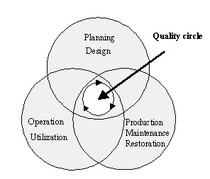
Fig. 1: Interaction of several phases during the lifetime
of a construction
Aim and purpose of any surveillance is the earliest possible detection of
a damage, failure or an injury to the safe operation of a construction in
order to be able to react appropriately and in time. However, surveillance
is only one of the columns of the stability and operational security of a
construction, which has to be seen in a holistic way (Fig. 2). Usually the
construction itself is the most important column. The activity and emergency
concepts include but are not limited to aspects of normative and budgetary
constraints; integrity, material and structure damage assessment;
intensified surveillance and diagnostic technologies; lifetime and
utilization evaluation; maintenance and repair, out-of-service and
replacement decisions etc. The worldwide immense number of in-service
structures requires more and more investments in these concepts. In Ger-many
for instance, these investments equal the capital expenditure for new
buildings in the very near future (SFB 477-2000). Under these circumstances
it is quite clear that surveillance and analysis techniques gain more and
more significance. Fig. 3 shows the result of a study in Japan which
analyzes the time elapsed between the completion of highway and railway
bridges and the detection of a damage. The study makes evident that the
knowledge of the integrity of in-service structures on a continuous time
basis is an ultimate objective for owners and maintenance authorities
(Bergmeister 2000).
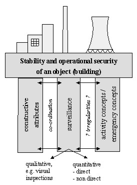
Fig. 2: Security concept for constructions
(Heunecke 2000)
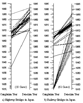
Fig. 3: Completion year and damage year of highway (a)
and railway (b) bridges in Japan (SFB 477-2000)
It is self-evident that engineering surveying cannot cover all aspects
but is capable of providing essential contributions. It has to cooperate and
communicate with other fields of engineering. A common basis for
communication is being provided and already applied by system theory.
The surveillance of an object involved in a deformation process requires
the object as well as the process to be modeled. Conventionally, geodetic
modeling the object (and its surrounding) means dissecting the continuum by
discrete points in such a way that the points characterize the object, and
that the movements of the points represent the movements and distortions of
the object. This means that (only) the geometry of the object is modeled.
Furthermore, modeling the deformation process means conventionally to
observe (by geodetic means) the characteristic points in certain time
intervals in order to monitor properly the temporal course of the movements.
This means that (only) the temporal aspect of the process is modeled. This
kind of modeling and monitoring an object under deformation in space and
time has been the traditional geodetic procedure (Fig. 4). (It is not the
scope of this report to discuss the methods of the various other disciplines
dealing with the measurement of geometrical object changes. Their
proceedings fit more or less the scheme of Fig. 4.) Consequently, the
deformations of an object are described solely in a phenomenological manner.

Fig. 4: Geodetic modeling of deformation processes in
space and time
For the analysis in space and time there are in principle two classes of
models. Models testing the identity or congruence of the geometrical
properties of an object at two (or more) points of time are referred to as
models of congruence. They regard the time factor only implicitly. Models
de-scribing the deformation on the basis of a given or assumed function of
time, i.e. velocity, acceleration etc., are called kinematic.
Practically, the classical deformation analysis consists in a purely
geometrical comparison of the state of an object (represented by its
characteristic points) at two different points of time. The model for the
analysis of the observations does not consider the time intervals between
the observations nor the factors responsible for the deformation -
explicitly. Implicitly, however, some knowledge and information about the
presumable behavior of the object and the deformations in space and time
have to flow into a proper set-up of the deformation monitoring project.
The only input quantities of the evaluation model are the geodetic
observables l, while the output quantities are the coordinates x of the
characteristic points at certain moments of time. Since the 1960s the
identity or the congruence of the point coordinates with respect to the
so-called null or initial epoch have been statistically investigated. The
procedure is such that a null-hypothesis is formulated requiring the
coordinates to be the same as before. This null-hypothesis is included into
the usual least-squares (LS) GAUSS-MARKOV model:
(1)
Crucial aspect is the statistic test of the so-called mean gap (global
test of congruence)
 , , 
(2)
(d vector of the coordinate differences,
Qdd
its cofactor matrix) on the basis of the probability relation
(3)
(Pelzer 1971). Basically the inherent differential
equation  is tested. is tested.
The global test detects whether there are any significant
coordinate differences. If there are any, then the next step is to localize
the point(s) which are causative. If need be, the movements of point
clusters can be generalized by rigid block movement or strain analysis, or
in terms of other systematic patterns. This kind of deformation analysis is
traditionally referred to as (conventional) deformation analysis, the
resulting point movement pattern as deformation model. Since this
‘geometrical’ deformation analysis (Chrzanowski et al. 1990) is based on the
hypothesis (1) of identical point coordinates, the deformation model is to
be called identity or congruence model (e.g. Welsch et al. 2000, pp.
369-418).
When automated measurement procedures came into use, the
temporal course of deformation processes was more and more considered in
evaluation models (e.g. Pelzer 1977b). If these models are restricted to the
investigation and description of object movements and distortions in space
and time, one speaks of kinematic models which have offered the opportunity
to extend the classical purely geometrical deformation analysis in
congruence models.
The intention of kinematic models is to find a suitable
description of point movements by time functions without regarding the
potential relationship to causative forces. Polynomial approaches,
especially velocities and accelerations, and harmonic functions are commonly
applied.
The relation of the space-time coordinates
x1
at an initial epoch t1 with respect to the coordinates
x2
at a consecutive epoch t2 are described by the time
dependent relation
 . .
(4)
 are the
mean velocity and acceleration of the points within the time interval
D
t. They represent the unknown parameters to be estimated. These
parameters are relevant to assess the process. The corresponding linearised
observation equation reads are the
mean velocity and acceleration of the points within the time interval
D
t. They represent the unknown parameters to be estimated. These
parameters are relevant to assess the process. The corresponding linearised
observation equation reads
 .
.
(5)
This system represents in general the set-up of a regression analysis. In
expansion of the basic regression analysis sequential adjustment algorithms
are an important mathematical tool which are in a formal manner a transition
to Kalman-filtering techniques, and are suitable to make use of consecutive
observations for updating and predicting the state of a process under
investigation (Pelzer 1987; Welsch et al. 2000, pp. 419-446).
4.
Dynamic Systems and
Advanced Deformation Analysis - Systematization of Deformation Models
Advanced evaluation models for deformation analysis do not only consider
the change of the geometry of an object in space and time. They rather
investigate and incorporate also the influencing factors (causative forces,
internal and external loads) causing the deformation. They regard in
addition the object's physical properties (material constants, extension
coefficients, etc.) which are characteristic and responsible for the
response of the object to the acting forces. The three elements 'acting
forces' as input signal, 'transmission through the object' as transfer
process, and 'response of the object' as output signal form a causal chain
or - according to the terminology of system theory - a dynamic process or a
dynamic system (Fig. 5).
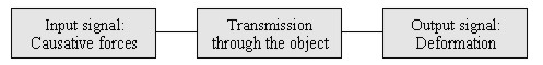
Fig. 5: Deformation as an element of a dynamic system
In recent years engineering sciences have established a standardized
mathematical description of the temporal behavior of dynamic systems
according to system theory. In the following the variants of dynamic systems
are characterized:
- Dynamic (cause-response) systems: Changes of input signals release a
time-dependent process of adaptation of the system with the consequence
that the reaction of the output side is delayed: a dynamic system has a
memory. This is the general case. Special cases can be distinguished with
respect to the factor time. There are two kinds of dynamic systems:
a) dynamic systems as such react as in the general case: the
deformations as the output signal are a function of time and (varying)
loads. The knowledge of the memory of the sys-tem is the basis for
prediction;
b) static systems can be seen as a special case of dynamic systems.
They react immediately (without a memory) to the change of the
causative forces: the new state is a state of equilibrium. The
deformations are a function of changed loads only.
- Autonomous (free) systems are not subject to acting forces. These
systems can nevertheless be in motion. There are two kinds of autonomous
systems:
c) kinematic systems are in motion; the motion can be described as
a function of time;
d) random walk systems are in motion, but the motion is random, a
function of time cannot be established apriori.
Modeling a dynamic process according to Fig. 5 is by far more
comprehensive than modeling solely the deformation as the reaction of the
object in space and time. The complexity of dynamic modeling makes the
requirement of interdisciplinary cooperation obvious.
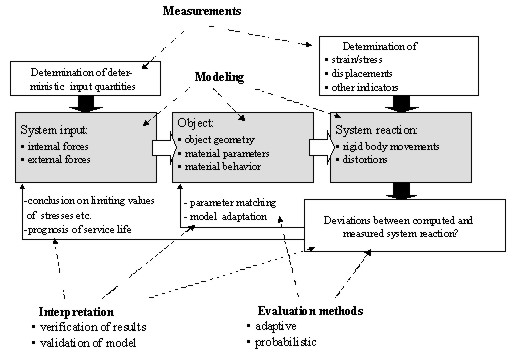
Fig. 6: Dynamic modeling of a construction
To set an example, the technical system 'construction' (Fig. 6) is
stressed by internal and external forces or loads (like traffic load, wind
pressure, backwater pressure, temperature etc.). These so-called input
quantities (input signal) have to be determined by measurements. The
reaction of the system is deformations (e.g. rigid body movements, strain).
In order to model (calculate, predict) the reaction of the system as the
output signal, the transmission through the object (transfer function) has
to be modeled as well. Parameters to do this are in particular the
construction's geometry, its material parameters and the assumed material
behavior. If the two elements - input signal and transfer function - are
known, the dynamic process can be modeled and the reaction can
quantitatively be predicted (if need be by the aid of the Finite Element
Method or another computation tool). This kind of a dynamic model is also
referred to as a deterministic (Chrzanowski et al. 1990), mechanical or
computational model. Consequently, error propagation should be taken into
consideration (e.g. Kuang 1993; Szostak-Chrzanowski et al. 1994; DIN
1319-1997). If, how-ever, in addition also the reaction of the system, i.e.
the deformations, is determined by (geodetic) measurements, the full
potentiality of dynamic models becomes obvious (integrated models). The
comparison of the predicted to the observed deformations may reveal some
deviations which are called 'innovation' (Fig. 10). The innovation is the
basic element for KALMAN-filtering techniques. Fig. 6 accentuates the
components of the investigation and the assessment of a process: modeling
the process (theory), performing the measurement of input and output
quantities, evaluating functional and stochastic relationships, and -
finally - assessing the findings by verification and validation. In this way
the model can be calibrated and the dynamic process be identified. Worldwide
numerous research centers are active to adapt and to apply this general
interdisciplinary scenario.
Summing up these comments and referring to the variants of dynamic
systems, according to sys-tem theory in principle the following four
categories of models can be distinguished for the evaluation of deformations
(Fig. 7):
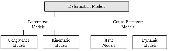
Fig. 7: Hierarchy of models in geodetic deformation
analysis (Welsch and Heunecke 1999)
Descriptive models like the congruence and kinematic models are already
described in par. 3. The class of cause-response models are the ones to be
characterized in the following in more details.
For many applications in our days the understanding of engineering
surveying intends - as out-lined above - to consider not only the space and
time domains of deformations, but rather the whole chain of a dynamic
process, i.e. to incorporate also the causative forces acting on the object
and the geometrical and physical properties of the object itself. With
today's technology the basic requirements thereto are available: the
possibility of measuring and recording the input and output signals of a
dynamic process are in the same way at hand as the computer capacities are
sufficient to perform the necessary algorithmic calculations. As practice
shows, in many instances the main difficulty is the availability of
appropriate software programs to process the data accordingly.
Static models describe the functional relationship between stress and
strain. Stress is caused by loads or the forces acting on the object and
resulting in strain as the object's geometrical reaction. Since the factor
time is not explicitly considered in static models, the object has to be
sufficiently in equilibrium in both the observation epochs, i.e. before and
after the load has been brought up on the object. Sufficiently in
equilibrium means, the object has to appear (more or less) motion-less
during the time of observation. The movements and distortions of the object
are considered a function of only the load but not the time. For static
models, the physical and geometrical structure, the material parameters and
other characteristic quantities of the object have to be known and to be
formulated in terms of differential equations expressing the stress-strain
relationship of the object. This requirement leads to another term of
characterization of static models: static models are parametric (see below),
structured or deterministic models. Other terms are state or theoretical
models; the evaluation applying static models is also called 'model
approach'. Static models are frequently applied, if the load-carrying
capacity of structures like bridges, pylons etc. is to be tested. An example
is given in par. 6.2.
Dynamic models are the most general and comprehensive models because they
aim to describe the reality of dynamic systems completely. The movements and
distortions of the object are considered a function of both load and time.
This implies time varying stresses and time varying re-actions. In contrast
to the static situation the object is permanently in motion. Monitoring such
a situation requires permanent and automatic observation procedures. Dynamic
models can be parametric or non-parametric (see below). Other terms for
non-parametric models are attitude or statistical, experimental or empirical
models; the evaluation applying non-parametric models is also called
'operational approach'. So far, there are hardly any parametric dynamic
models being used for the geodetic analysis of dynamic processes, at least
not for the so-called multiple input - multiple output (MIMO) situations.
Almost all dynamic models applied to deformation analysis are
non-parametric.
In Fig. 8 the four categories of deformation models are characterized by
their capacity of taking the factors 'time' and 'load' into account.
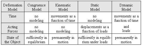
Fig. 8: Characterization and classification of
deformation models (Welsch and Heunecke 1999)
In system theory, the set-up of an appropriate mathematical-physical
representation of the transfer function of a dynamic system is called system
identification. System identification can be achieved, if the input as well
as the output signals are available as measured quantities. The feasibility
of how a model for the transfer function can be set up, is decisive for the
choice of a parametric or a non-parametric identification (e.g. Heunecke et
al. 1998, Heunecke and Welsch 2000), see Fig. 9.
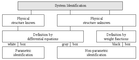
Fig. 9. Methods of system identification (Heunecke 1995;
Welsch 1996)
If the physical relationship between input and output signals, i.e. the
transmission or transfer process of the signals through the object or - in
other words - the transformation of the input to out-put signals, is
supposed to be known and can be described by differential equations, then
the model is called a parametric model (structural model). The system
identification is carried out in a so-called 'white box' model. Of course,
white box models are - as it is the case with all models - an idealization
of the real world.
The fundamental equation of any dynamic model of a system (Welsch et al.
2000, pp. 461-474) is the differential equation of linear dynamic
elasticity:
 (6)
(6)
y(t) is the system input, the acting
forces which have, if need be, to be complemented by the disturbance noise;
x(t) and its derivatives are the system output (to be
monitored e.g. by geodetic means); the matrices K, D,
and M
contain - in case of an application of mechanics like a building or another
construction - material and design parameters for rigidity, damping and
mass. Depending on the actual problem individual sets of parameters or
measurements can be inapplicable. For instance, for the investigation of
characteristic oscillations the damping matrix is to be omitted, and with
slow motions the mass can be neglected (Heunecke 1995, Jaeger et al. 1997).
For static models (Welsch et al. 2000, pp. 447-459) the
special case of a dynamic model
 (7)
(7)
is applicable. Static systems are characterized by
capturing a new state of equilibrium after assuming a load with y(t)
= const.
As a trivial form the case
 (8)
(8)
is of special interest. It comprises the models of
identity and congruency, i.e. the most common application of deformation
monitoring based on geodetic networks; see par. 3.
In the context of structural models it is of importance, that coordinate
systems are introduced as reference systems. Coordinates are intermediate
quantities of the evaluation procedure. They are called state parameters
comprised in the state vector. Apart from coordinates also additional
(physical) state parameters may be used. In the sense of system theory state
parameters serve for the description of the inherent relations of the
system; they form the state space. The investigation of a dynamic process
with the help of a structural model is based on the analysis of the state
space.
If with parametric system identification only the time dependence rather
than the local variation of the process is considered, the system can be
defined by 'lumped parameters'. Ordinary differential equations are
sufficient in this case. If with parametric system identification apart from
the time dependence also the local variation of the parameters is
considered, the system has to be defined by 'distributed parameters'. This
leads to partial differential equations. If the differential equations are
set up for restricted areas only, the partial differential equations can be
replaced by ordinary differential equations which are, however, effective
only within these limited areas (local discretisation). The solutions found
for the individual areas have to be joined to each other taking into account
boundary conditions for a smooth connection. The result represents an
approximate solution of the original differential equation. A numerical
procedure is given by the Finite Element Method (FEM) which is today the
standard computation method for any kind of structural problems in civil
engineering and in many other engineering sciences.
KALMAN-filtering is the most popular and universal estimation tool for
system identification and can be applied to all kinds of models in Fig. 7
and 8, resp. (Welsch et al. 2000, pp. 285-317). The essential idea can be
explained as follows. On the one side there is the theory modeling the
object by differential equations. These equations form the so-called system
equation. On the other side there are measurements monitoring the real
behavior of the object. The measurements are formulated as the so-called
observation equation. KALMAN-filtering is a technique to combine both
equations by least squares adjustment in order to gradually improve the
identification of the sys-tem. For this the innovation, i.e. the difference
between the predicted and the measured reaction of the object, is essential.
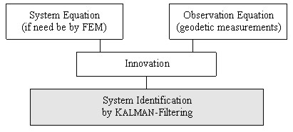
Fig. 10: Substance of KALMAN-filtering (Heunecke 1995)
Input quantities Y of a Kalman-filtering
process are the previous state vector
xk
at
time tk, the deterministic input quantities
uk
(acting forces), the disturbance quantities
wk
and the monitoring observations
lk+1
including the respective covariance matrices:
 . .
(9)
The quantities of main interest X are the
already mentioned innovation dk+1, the
filtered (updated) state vector  and the residuals
 and and
 . These quantities can be
computed through the linear equation (10) with respect to the predicted
state vector . These quantities can be
computed through the linear equation (10) with respect to the predicted
state vector  and the observations lk+1;
Kk+1
is the so-called gain-matrix and
Dk+1 is the
covariance matrix of the innovation:
and the observations lk+1;
Kk+1
is the so-called gain-matrix and
Dk+1 is the
covariance matrix of the innovation:
 . .
(10)
The algorithm can be used whenever a system equation can
be established. In a congruence model the system equation degenerates to the
prognosis of identical coordinates; deterministic input quantities
uk
are not modeled. For a kinematic approach the state vector contains
coordinates, velocities and accelerations. Kalman-filtering in deformation
analysis is mainly applied to static or dynamic models with system equations
set up by the Finite Element Method, see par. 6.2.
5.2 Non-parametric models
If there is no way of modeling the geometrical and the
physical structure of a system, the relationship between input and output
signals can be formulated only in the sense of regression and/or correlation
analysis (behavior model). Time series analysis is helpful. System
identification means then the determination (estimation) of the
regression/correlation coefficients. Commonly these coefficients or kernels
are called parameters, too, although they are not the physical parameters of
the process under investigation; they relate rather the input signals to the
output signals without any physical significance. These non-parametric
models are therefore also called ‘black box’ models. It means that system
identification is based on measurements only but not on a mechanical model;
it is symptom but not model orientated.
The most general description of non-parametric models is
a set of partial differential equations. In the case of a ‘single input –
single output model’ (SISO) it is given by an ordinary differential equation
which can be established (Ellmer 1987; Welsch 1996) by the approach
 . .
(11)
If one proceeds from the differential to a difference
equation, the model is also known as the so-called ARMA (autoregressive
moving average) model:
 . (12) . (12)
The unknown coefficients
ak and
bk
are the parameters to be estimated in the identification procedure. The
boundary values q and p represent the continuance of the
memory: at time tk the model recollects all the input and
output events back to those boundaries.
Characteristic for this elementary non-parametric model
is the fact, that for q > 3 and p > 0 a physically meaningful
model structure gets lost, although the coefficients have to be regarded as
functions of the material and design parameters of the system. For q
£ 3 and p = 0, however, the parameters can physically be
interpreted. In other cases the model is a ‘gray box’. However, the
distinction between the different kinds of models – white, gray and black –
is gradual, and depends on the appreciation of terms like ‘parameter’ or
‘physical structure’.
The ARMA-model consists of a recursive and a
non-recursive part:
 .
(13) .
(13)
For p = 0 the model is autoregressive: the actual
observation xk is considered a linear combination of the
past observations and the present system input yk. For
q
= 0 the model becomes non-recursive: the actual system output is a linear
combination of the present and the past system inputs. The coefficients
bj
can then be regarded as the factors of a regression analysis.
For continuous observations the representation of the
non-recursive (linear) model is the convolution integral (Strobel 1975)
 ,
(14) ,
(14)
where  is
the so-called weight function which plays - as above - the role of
regression analysis parameters. is
the so-called weight function which plays - as above - the role of
regression analysis parameters.
For the treatment of non-linear unstructured problems for
instance the so-called Volterra-model (Wernstedt 1989) has been developed:
 (15)
(15)
+ higher order terms.
In the discrete case these models can be written in form
of a summation or multiple summation equation, resp. (Pfeufer 1990, 1993).
Non-parametric models can be applied to a great variety of systems and
processes.
Time series analysis (Welsch et al. 2000, pp. 319-367) as
such is another method of system identification and is frequently applied in
non-parametric situations. The most significant information to be calculated
in the time domain of a time series is its expectation value and the
auto-covariance function which informs of variance of the process observed.
Comparing the input and the output time series by calculating the
cross-covariance function, one obtains information about the correlation of
the two time series and whether the reaction of the system is delayed with
respect to the input signal (phase shift). If one applies
Fourier-transformations to switch from the time to the frequency domain,
characteristic frequencies of the process can be detected. The output signal
comprises only frequencies which are also contained in the input signal.
Consequently, frequencies which are in the output but not in the input
signal, can give clues that there may be more than the investigated factors
influencing the system. Time series analysis as such
has a wide range
of applications in geodetic deformation analysis (e.g.
Kuhlmann 1996).
Recently new analysis techniques have been adopted from
control engineering: neural networks and fuzzy logic have been used to set
up models for the identification of input-output systems (Heine 1999).
In practice, a comprehensive and complete analysis of a deformation
process can hardly be carried out applying only one kind of the above
mentioned models. In almost all instances, experiments have to be made to
find the best method and procedure, even 'trial and error' should not be
excluded. This is especially relevant, if the geometrical and/or physical
model to be chosen is not clear but questionable so that the problem of
model separability arises (Lu 1987, Chen and Chrzanowski 1994). This point,
however, is not specified further on in detail.
A practical approach may be the following: According to Chrzanowski et
al. (1990) the integrated analysis of deformation surveys includes the
geometrical analysis of the status of the deformable body and the physical
interpretation, i.e. the identification of the dynamic process. Fig. 11
shows an idealized flowchart of the integrated deformation analysis.
'Integrated' means the combination of the geometrical analysis with
prediction models.
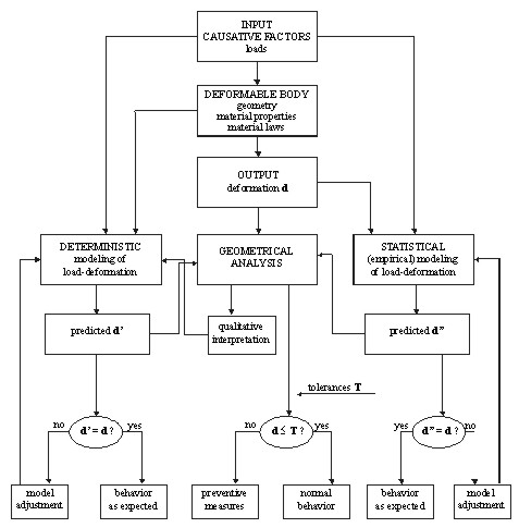
Fig. 11: Flowchart of integrated deformation analysis
(Chrzanowski et al. 1990)
The latter can be achieved by applying either the 'statistical', i.e. the
non-parametric, or the 'deterministic', i.e. the parametric, method. Once
the load-deformation relationship is established, the results may be used
for the development of prediction models. Through the comparison of
predicted deformations with the results of the geometrical analysis of the
actual deformations, i.e. the innovation, a better understanding of the
mechanism of the dynamic system is possible. The new knowledge can be used
in 'model adjustments' the results of which lead iteratively to what has
been referred to (Fig. 6) as parameter matching and model adaptation.
A typical example for the application of parametric modeling of a dynamic
system is load trials on constructions. The static behavior of a 10.0 m x
2.0 m shell structure, made of bricks, was investigated (Hesse et al. 2000).
The semilateral surface loading (1.0 kN/m², loading step No. 6) of the
structure and the settlements predicted using FEM is shown in Fig. 12. The
surface loading was stepwise increased from zero up to 4.0 kN/m2 (loading
step No. 24). The envisaged break-down of the structure could, however, not
be achieved. For two of the monitored points (No. 13 and No. 33) the
predicted settlements (ANSYS, system equation) and the displacements
measured by means of leveling and extensometers (observation equation) are
depicted in Fig. 13. The discrepancy between the prediction and the
measurements, in terms of KALMAN-filtering the 'innovation', is quite
striking.
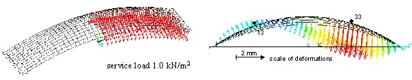
Fig. 12: Semilateral loading of a shell construction and
predicted settlements (Hesse et al. 2000)
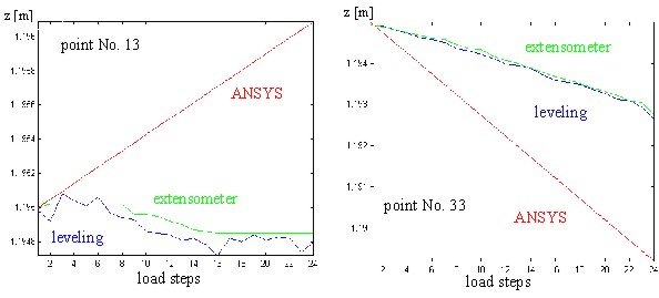
Fig. 13: Comparison of predicted and measured settlements
of points No. 13 and 33 (Hesse et al. 2000)
Fig. 14: Settlements of points No. 13 and 33 after the
adaptive filtering process (Hesse et al. 2000)
After adaptive KALMAN-filtering the innovation is reduced so that the
predicted and filtered settlements are in accordance with the measured
values (Fig. 14), there is no significant difference anymore. Adaptive
filtering means to identify, i.e. to estimate the material parameters
(Young's modulus) of the structure as additional unknown state parameters
(state vector augmentation). As a result, the material parameters (physical
state quantities) obtain values which differ quite a bit from the original
assumptions. Based on the results of the parametric identification, the
assessment of the stability and the operational security of the structure is
now much more realistic and reliable then it was before.
The following example discusses the reaction of the foundation pillars of
a large turbo engine due to temperature variations (Ellmer 1987). Due to
irregularities and major gaps during the data acquisition of the temperature
and deformation measurements, in a first step interpolation and
approximation procedures were applied to the time series in order to achieve
equispaced data which are required for the analysis models.
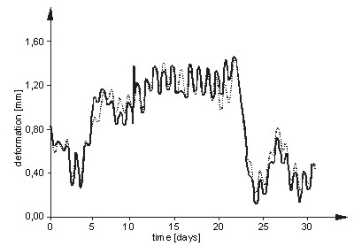
Fig. 15: Measured (¾ ) and
modeled (× ×
×
) deformation of a pillar supporting the turbine table
In a second step Fourier transformations were used to get preliminary
information on the behavior of the system. The last step relates the
temperature changes to the deformations by a SISO identification model which
considers the fact that temperature changes effect the foundation pillars
over a longer period of time. This model is given by equation (13)
which is restricted, however, to the estimation of the non-recursive
parameters b0, ... , bp only, where p
stands for the memory-length. The solution includes p
= 30 significant parameters bk. This model is able to
demonstrate that most of the deformations can be explained by the recorded
temperature variations (Fig. 15).
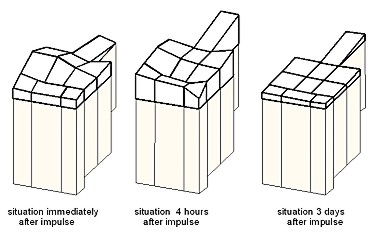
Fig. 16: Deformation of the table plate as caused by a
unit impulse of 1 K ( × = 0,01 mm)
Fig. 16 depicts the reaction of all the pillars of the turbine table to
an input impulse of 1 K immediately after the impulse, after 4 hours and
after 3 days. The point of this sort of non-parametric system identification
is that the model describes the reaction of the object to be monitored in a
'black box' manner. It is meaningful, because it relates input signals
(temperature variations as physical causative forces) to output information
(deformations of the pillars). It does not contain, however, any information
about the structure or at least the significant material parameters, e.g.
the coefficient of expansion, of the system which could make evident why the
system reacts as it obviously does. The physical interpretation of dynamic
processes on the basis of non-parametric models is therefore always limited;
the interpretation is symptom oriented.
Another typical application of deformation analysis is ground subsidence.
The Sparwood coal fields, British Columbia, for instance were observed and
analyzed by Chrzanowski et al. (1990). The purpose of the surveys was to
monitor ground movements caused by the extraction of a 200 m by 700 m panel
of a 12 m thick and steeply inclined coal seam (Fig. 17). Three types of
monitoring observations were used under rough climate conditions:
tacheometric geodetic measurements, aerial photogrammetric surveys and
continuous measurements of changes of ground tilts by automated biaxial
tiltmeters. Between 1980 and 1982 the panel extraction (input quantity)
produced displacements of up to 2.5 m with surface cavings near the coal
outcrop and cracks at the mountain ridge. The best fit model of the
displacement field of the complicated deformation pat-tern (Fig. 18) was
obtained by applying the combined analysis of all three types of
observations (Chrzanowski et al., 1986). The analysis led to a suspicion
that there was either a geological fault or a discontinuity in the rock mass
was created by the progressing mining activity.
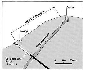
Fig. 17: Cross-section of the subsidence area
(Chrzanowski and Szostak-Chrzanowski, 1986)
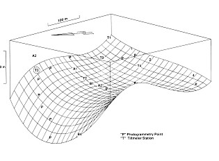
Fig. 18: Ground subsidence model obtained from geodetic,
photogrammetric and tiltmeter measurements (Chrzanowski et al. 1990)
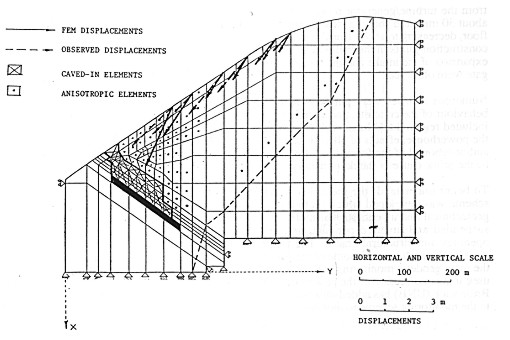
Fig. 19: FEM displacements versus observed values in the
Sparwood coal fields
(Chrzanowski and Szostak-Chrzanowski, 1986)
The phenomenon as a whole could not be readily explained. Therefore, a
deterministic FE modeling of the subsidence was performed (Chrzanowski and
Szostak-Chrzanowski 1986). The modeling was difficult due to the fact that
besides the unknown fault parameters also the values of the in situ Young's
modulus of the rock were not well known. However, using the results of the
geometrical analysis, the deterministic model could be calibrated
(adaptation of Young's modulus, insertion of the assumed fault parameters
into the analysis). Two FE models were analyzed: one without the assumed
discontinuity and one with the insertion of the suspected fault. The FEM
results with the fault gave incomparable better agreement with the observed
values of the displacements. The final result obtained from this static
model is shown in Fig. 19. The findings of the integrated analysis led to
the closing of the mining operation to prevent a potential slope failure.
The example demonstrates that parametric description, i.e. deterministic
modeling, of geological phenomena, though difficult to perform, may lead to
useful physical interpretation of deformations if properly combined
(calibrated) with the geometrical model. Apart from parameter matching
according to Fig. 6 also the identification of the unknown structural
properties as for instance the fault zone geometry is crucial for an
appropriate solution.
For many reasons the development and application of dynamic models is of
great significance for the investigation of technical and natural phenomena.
They offer the most far-reaching possibilities for the analysis,
interpretation and the prognosis of processes which are essential aspects of
deformation analysis. Therefore, evaluation procedures are to be aimed at
which are able to fulfil the following essential tasks:
- processing of big amounts of data gathered by different sensor systems
(hybrid data) monitoring the input and output signals of a dynamic system
- identification of the system behavior applying models which are
adequate with respect to the process to be monitored
- treatment of disturbing influences by filtering
- prediction of the reactions of the system, if it acts regular
- assessment of the reaction of the system, if it undergoes irregular or
even extreme influences
- separation of the influences caused by the individual input factors
- determination of the main influencing factors
- possibility to control the process via factors which are controllable
- optimization of monitoring and observation plans due to a better
knowledge of the process
- comprehensive interpretation of the results achieved due to the
knowledge of identifiable and physically well-founded parameters of the
process.
In many cases there exists only poor knowledge of the internal and
external connections of a process. Therefore a universal, generally accepted
single scheme for the investigation of different objects cannot be set up.
The numerous classes of dynamic models as discussed in this report offer,
however, a great variety of possibilities for a pertinent treatment of a
great number of processes and objects. The development in this domain has
been pushed forward considerably in the previous years, and will be advanced
in the future.
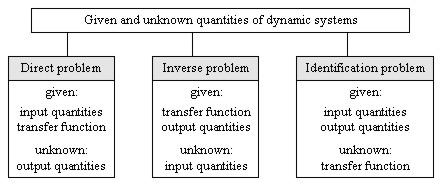
Fig. 20: Essential problems of dynamic systems (after
Natke 1983)
System analysis (direct problem) requires the input quantities and the
transfer function to be known. The reaction of the system is in this case
the unknown quantity. At last, the identification problem derives the
transfer function from observed input and output signals.
The following general problems can be treated and solved for with the
help of dynamic modeling (Fig. 20). In case of the direct or design problem,
the system behavior (transfer function) is regarded to be known, so that the
output signal can be computed (predicted). The inverse problem (back
analysis, reverse engineering) assumes the reaction and the transfer
function as given and analyses the causative factors (e.g. Kersting 1992).
From the geodetic point of view a contribution can be given to system
identification by verifying the system's behavior on the basis of input and
output signals to be measured. Transitions between the three general
problems are fluent.
System identification is performed to determine the physical status of a
deformable body, the state of internal stresses and, generally, the
load-deformation or stress-strain relationship. Once this relationship is
established, the results (system equation) may be used for the development
of a prediction model. Through the comparison of predicted deformations with
the result of the geodetic analysis of the actual deformations (observation
equation), a better understanding of the mechanism of the deformations is
achieved. Thus, engineering surveying may significantly con-tribute to a
realistic interpretation of a dynamic process under investigation.
On the other hand, the prediction models which, in most cases, are
developed by other specialists, supply important information to the
surveying engineer about the deformations to be expected, facilitating the
design of the monitoring scheme as well as the selection of the deformation
analysis model in the geometrical realm. Unfortunately, in many cases this
scenario of a truly interdisciplinary approach to the design and analysis of
deformation surveys has not yet been implemented in practice. The reasons
are an inadequate understanding of the methods of system identification by
surveying engineers, and an inadequate familiarization of other specialists
with the comparatively new methods of advanced geodetic analysis of dynamic
processes. The gain of knowledge to be achieved by the combination of
techniques developed in system theory like KALMAN-filtering with techniques
applied in civil engineering like FEM and engineering surveying, e.g.
statistical testing procedures and reliability considerations, offers new
aspects for the future.
Within the last few years, one can see some progress in the right
direction, not only within the geodetic community, with more scientific
papers on the identification of dynamic systems presented at surveying and
geodetic meetings, but in the meantime also at conferences of other
disciplines. However, these developments must be intensified. The trend will
be supported and enhanced by a commonly acknowledged terminology. The
potentiality of all the possibilities of analyzing dynamic systems by
appropriate models and methods - from geometrical descriptions to highly
sophisticated integrated models and analysis techniques - has to be
exploited.
Ad-Hoc Committee of FIG (1993) under the leadership of A.
Pfeufer: G. Milev, W. Proszynski, G. Steinberg, W.F. Teskey, W. Welsch:
Report of the Ad-Hoc Committee on Classification of Deformation Models and
Terminology. 7th International FIG-Symposium on Deformation
Measurements. Department of Geomatics Engineering, The University of
Calgary, Alberta. Proceedings, pp. 66-76
Ad-Hoc Committee of FIG (1994) under the leadership of A.
Pfeufer: G. Milev, W. Proszynski, G. Steinberg, W.F. Teskey, W. Welsch:
Classification of Models for the Geodetic Examination of Deformations.
Perelmuter Workshop on Dynamic Deformation Models. The Technion, Haifa,
Israel. Proceedings, pp. 94-108
Bergmeister, K. (2000): Integrated Monitoring of Bridges.
Colloquium of SFB 477, Technical University Braunschweig, Germany.
22.06.2000
Boljen, J. (1983): Ein dynamisches Modell zur Analyse
und Interpretation von Deformationen. Wissenschaftliche Arbeiten der
Fachrichtung Vermessungswesen der Universität Hannover, No. 122
Boljen, J. (1984): Statische, kinematische und dynamische
Deformationsmodelle. Zeitschrift für Vermessungswesen 109, pp.
461-468
Bonn (1978): 2nd International Symposium on
Deformation Measurements. Bonn, 25.-28.09.1978. Hallermann, L. (ed.):
Vermessungswesen
Band 6. K. Wittwer, Stuttgart
Chen, Y.Q. (1983): Analysis of Deformation Surveys - A
Generalised Method. Department of Surveying Engineering, University of
New Brunswick. Technical Report No. 94
Chen, Y.Q. and A. Chrzanowski (1994): An Approach to
Separability of Deformation Models. Zeitschrift für Vermessungswesen
119, pp. 96-103
Chen, Y.Q. and A. Chrzanowski (1986): An Overview of the
Physical Interpretation of Deformation Measurements. Deformation
Measurements Workshop Modern Methodology in Precise Engineering and
Deformation Surveys - II. MIT, Cambridge, Mass., USA. Proceedings,
pp. 207-220
Chrzanowski, A. (1981) with contributions by members of
the FIG Ad-Hoc Committee: A Comparison of Different Approaches into the
Analysis of Deformation Measurements. FIG-XVI Congress, Montreux,
09.-18.08.1981. Proceeding, paper 602.3
Chrzanowski, A. (1992): Recommendations. 6th
International FIG-Symposium on Deformation Measurements.
Wissenschaftliche Arbeiten der Fachrichtung Vermessungswesen der Universität
Hannover,
No. 217, Hannover 1996
Chrzanowski, A. (1999): Review of Activity FIG Working
Group 6.1 Concerning Methods of Deformation Analysis and Classification of
Deformation Models. 9th International FIG-Symposium on
Deformation Measurements, Olsztyn, 27.-30.09.1999. Proceedings,
pp. 410-415
Chrzanowski, A., Y.Q. Chen, J. Secord (1982): On the
Analysis of Deformation Surveys. 4th Canadian Symposium on Mining
Surveying and Deformation Measurements. The Canadian Institute of Surveying,
Banff, 07.-09.06.1982. Proceedings
Chrzanowski, A., J. Secord (1983): Report of the Ad-Hoc
Committee on the Analysis of Deformation Surveys. XVII. FIG-Congress,
Toronto, 01.-11.06.1983. Proceedings, paper 605.2
Chrzanowski, A., Y.Q. Chen (1986): Report of the Ad-Hoc
Committee on the Analysis of Deformation Surveys. XVIII. FIG-Congress,
Toronto, 01.-11.06.1986. Proceedings, paper 608.1
Chrzanowski, A., Y.Q. Chen, P. Romero and J. Secord
(1986): Integration of Geodetic and Geotechnical Deformation Surveys in
Geosciences. Tectonophysics 130, pp. 369-383
Chrzanowski, A., A. Szostak-Chrzanowski (1986):
Integrated Analysis of Ground Subsidence in a Coal Mining Area: A Case
Study. Deformation Measurement Workshop, Mass. Institute of Technology,
31.10. – 01.11.1986. MIT, Cambridge, Mass., USA. Proceedings, pp.
259-274
Chrzanowski, A., Y.Q. Chen, A. Szostak-Chrzanowski, J.M.
Secord (1990): Combination of Geometrical Analysis with Physical
Interpretation for the Enhancement of Deformation Modelling. XIX. FIG
Congress, Helsinki 1990, Proceedings, Com. 6, pp. 326-341
DIN 1319, Part 4 (1997): Basic Concepts of
Measurements, Treatment of Uncertainties in the Evaluation of Measurements.
German Standard
Ellmer, W. (1987): Untersuchung temperaturinduzierter
Höhenänderung eines Großturbinentisches. Schriftenreihe des Studiengangs
Vermessungswesen, Universität der Bundeswehr München, No. 26, Neubiberg
Felgendreher, N. (1981): Studie zur Erfassung und
Verarbeitung von Meßdaten dynamischer Systeme. Deutsche Geodätische
Kommission, Reihe B, No. 256, München
Felgendreher, N. (1982): Zu Modellierungsproblemen bei
dynamischen Systemen. Zeitschrift für Vermessungswesen 107, S.
125-129
Heck, B., J.J. Kok, W. Welsch, R. Baumer, A. Chrzanowski,
Y.Q. Chen, J.M. Secord (1982): Report of the FIG Working Group on the
Analysis of Deformation Measurements. In: I. Joó and A. Detreköi (eds.):
Deformation Measurements, pp. 337-415. Akademiai Kiadó, Budapest
Heine, K. (1999): Zur Beschreibung von
Deformationsprozessen durch Volterra- und Fuzzy-Modelle sowie Neuronale
Netze. Deutsche Geodätische Kommission, Reihe C No. 516, München
Hesse, C., O. Heunecke, M. Speth, I. Stelzer (2000):
Belastungsversuche an einem Schalentragwerk aus Ziegelsteinen. In:
Schnädelbach und Schilcher (Hrsg.): XIII. Internationaler Kurs für
Ingenieurvermessung München, 13.-17. 03. 2000. Proceedings, pp.
340-345
Heunecke, O. (1995): Zur Identifikation und
Verifikation von Deformationsprozessen mittels adaptiver Kalman-Filterung
(Hannoversches Filter). Wissenschaftliche Arbeiten der Fachrichtung
Vermessungswesen der Universität Hannover, No. 208
Heunecke, O., H. Pelzer, W. Welsch (1998): On the
Classification of Deformation Models and Identification Methods in
Engineering Surveying. XXI. FIG-Congress 1998, Brighton. Proceedings,
Com. 6, pp. 230-245
Heunecke, O. (2000): Ingenieurgeodätische Beiträge zur
Überwachung von Bauwerken. Workshop ‘Dynamische Probleme – Modellierung und
Wirklichkeit’, Hannover, 05.-06.10.2000. Proceedings, pp. 159-176
Heunecke, O., W. Welsch (2000): A Contribution to
Terminology and Classification of Deformation Models in Engineering Surveys.
Journal of Geospatial Engineering, vol. 2. No. 1, pp. 35-44, Hong
Kong
Jaeger, R., U. Haas, A. Weber (1997): Ein ISO 9000
Handbuch für Überwachungsmessungen. Schriftenreihe des Deutschen Vereins
für Vermessungswesen No. 27, pp. 415-427, K. Wittwer
Kersting, N. (1992): Zur Analyse rezenter
Krustenbewegungen bei Vorliegen seismotektonischer Dislokationen.
Schriftenreihe des Studiengangs Vermessungswesen der Universität der
Bundeswehr, No. 42, Neubiberg
Krakow (1975): 1st International Symposium on
Deformation Measurements by Geodetic Methods. FIG Commission 6 (Ed.):
Krakow, 22.-24.09.1975. Proceedings
Kuang, S. (1993): A Methodology for the Accuracy Analysis
of the Finite Element Computations Applied to Structural Deformation
Studies. Allgemeine Vermessungsnachrichten, International Edition,
vol. 10, pp. 1-14
Kuhlmann, H. (1996): Ein Beitrag zur Überwachung von
Brückenbauwerken mit kontinuierlich registrierten Messungen.
Wissenschaftliche Arbeiten der Fachrichtung Vermessungswesen der Universität
Hannover, No. 218
Lu, G. (1987): On the Separability of Deformation Models.
Zeitschrift für Vermessungswesen 112, pp. 555-563
Natke, H.G. (1983): Einführung in Theorie und Praxis
der Zeitreihen- und Modalanalyse. Vieweg und Sohn,
Braunschweig-Wiesbaden
Pelzer, H. (1971): Zur Analyse geodätischer
Deformationsmessungen. Deutsche Geodätische Kommission, Reihe C, No.
164, München
Pelzer, H. (1977a): Zur Analyse von permanent
registrierten Deformationen. VII. Internationaler Kurs für
Ingenieurvermessungen hoher Präzision, Technische Hochschule Darmstadt,
29.09.-08.10.1976. Proceedings, pp. 781-796
Pelzer, H. (1977b): Ein Modell zur meßtechnischen und
mathematischen Erfassung kontinuierlicher Deformationsvorgänge. XV.
FIG-Congress, Stockholm 1977. Proceedings, paper 607.1
Pelzer, H. (1978): Geodätische Überwachung dynamischer
Systeme I. 2nd International Symposium on Deformation
Measurements. Bonn, 25.-28.09.1978. Hallermann, L. (ed.):
Vermessungswesen, Band 6, paper 60. K. Wittwer, Stuttgart
Pelzer, H. 1987: Deformationsuntersuchungen auf der Basis
kinematischer Modelle. Allgemeine Vermessungs-Nachrichten 94, pp.
49-62
Pfeufer, A. (1990): Beitrag zur Identifikation und
Modellierung dynamischer Deformationsprozesse. Vermessungstechnik 38,
pp. 19-22
Pfeufer, A. (1993): Analyse und Interpretation von
Überwachungsmessungen - Terminologie und Klassifikation. Zeitschrift für
Vermessungswesen 118, pp. 470-476
SFB 477 (2000): Collaborative Research Center: Life Cycle
Assessment of Structures via Innovative Monitoring. Technical University of
Brunswick.
http://www.sfb477.tu-bs.de
Szostak-Chrzanowski, A., A. Chrzanowski, Y.Q. Chen
(1994): Error Propagation in the Finite Element Analysis of Deformations.
XX. FIG Congress, Melbourne 1994. Proceedings, paper 602.4
Teskey, W.F. (1986): Integrated Analysis of
Deformations. Open File Report to the Department of Surveying
Engineering, University of Calgary, Alberta, Canada
Teskey, W.F. (1988): Integrierte Analyse geodätischer
und geotechnischer Daten sowie physikalischer Modelldaten zur Beschreibung
des Deformationsverhaltens großer Erddämme unter statischer Belastung.
Deutsche Geodätische Kommission, Reihe C, No. 341, München
Welsch, W. (1996): Geodetic Analysis of Dynamic
Processes: Classification and Terminology. 8th International
FIG-Symposium on Deformation Measurements, Hong Kong, 25.-28.06.1996.
Proceedings,
pp. 147-156
Welsch, W., O. Heunecke (1999): Terminology and
Classification of Deformation Models. 9th International
FIG-Symposium on Deformation Measurements, Olsztyn, 27.-30.09.1999.
Proceedings,
pp. 416-429
Welsch, W., O. Heunecke, H. Kuhlmann (2000):
Auswertung geodätischer Überwachungsmessungen, 510 pp. Wichmann Verlag,
Heidelberg
Wernstedt, J. (1989): Experimentelle Prozeßanalyse.
R. Oldenbourg Verlag, München-Wien
|


